Chapter 3 Reliability in poverty measurement

Abstract

This chapter introduces the theory and concept of reliability. An intuitive explanation is provided at the beginning of the chapter to underline the implications of reliability for measurement. Then, a formal introduction to the theory of reliability is provided. Reliability can be estimated using different approaches, the chapter discusses its limitations. The second main section of the chapter illustrates how reliability works and how can it be estimated using R and Mplus by using simulated data. Then a real-data example is used to show some of the typical problems involved in the examination of reliability.

3.1 Intuition to the concept of reliability

In what sense the concept of reliability relates to the idea of having a measure we can trust? Poverty analysts and policymakers require indices they believe in to focus on more important issues like developing and studying poverty eradication strategies. There is nothing worse in measurement that a scale that causes disbelief in that the debate concentrates upon how bad a measure is and not upon how good or bad a policy is. `Trust’ is built upon consistent and meaningful estimates. For example, imagine a case in which we could conduct two surveys to the same population. Ideally, we expect to find that the response patterns remain unchanged from \(t_1\) to \(t_2\). This is telling us that our index is stable across samples. A noisy index, in contrast, would lead to unstable responses and it is impossible to distinguish a signal (the thing we are interested in) from noise (unnecessary and confusing variability). However, consistency is not simply having the same response patterns ceteris paribus across two samples. The main implication for measurement of consistency is that we will get systematic population orderings, i.e. people ranked with very low (latent) living standards should remain in the same position across different measurements⁴.

One useful way to think about reliability in measurement is by imagining what would happen to our population orderings when we have good and bad indicators. Imagine a case in which one of the deprivation indicators is not a good measure of poverty, like having a folding bicycle. This variable will have a low correlation with the rest of the deprivation indicators. Spearman (1904)’s theory of reliability (or attenuation) tells us to be suspicious about such kind of behaviour. The problem is that low correlation (or even worse negative correlation) could mean that the indicator in question in not a consequence by poverty (“Lack of command of resources over time” See Chapter 1). The effect of bad indicators is that we will end up with two different population rankings depending on whether we include folding bicycle in our index. How different? It will depend upon how poorly correlated the indicator in question is with the rest and how good the rest of indicators is as a whole -i.e. how reliable these are-. Therefore, even with a very similar response pattern, our scale will be rather unstable to be trusted. Of course, if we know that the folding bicycle item is an unreasonable measure of poverty, we would have drop it before the empirical analysis. However, as we will see with some examples, in poverty measurement there are variables or thresholds of these variables that are quite contested.

Now imagine a different scenario where we have only good outcome measures of poverty and, for some reason, a good variable like lacking drinking piped water inside the house is dropped from the index (assuming this is a developing country where this measure works!). If we drop this indicator from our analysis, we would lose valuable information. Making the signal weaker is not as difficult as it might seem. Lack of good quality data or bad theories will increase the risk of missing some good indicators. Therefore, we would like that our scale is protected against the perils of real-data analysis. In other words, we would like to have a measure that is not too sensible to information losses. Reliability theory aims at this kind of scenario. That, indeed, put us in a position of producing measures we can trust. High reliability is a property that, for instance, protects an index against certain information losses, i.e. the higher the reliability, the lower the effect of missing variables. Yet, missing indicators could be damaging for policy reasons, of course.

3.2 Reliability theory

Reliability is a key concept in measurement theory and can be simple defined as the homogeneity of an index (Revelle & Zinbarg, 2009). A homogeneous index is a scale whose indicators are manifestations of the same trait, which is why from Spearman (1904)’s theory we expect them to be correlated as they are caused by the same phenomenon⁵. In the literature, several authors refer to reliability as internal consistency of an index because this a consequence of homogeneity. How this term of homogeneity relate to our intuition about reliability? In the example above having an indicator that is not a good measure of poverty means that the index is heterogeneous -i.e. there is more than more phenomenon causing deprivation- and therefore leads to inconsistent population orderings. Thus at the core of the principle of reliability lies the idea of having a series of items that would have a predictable behaviour when aggregated, i.e. if an index is reliable we should expect to have very similar population rankings across samples or small variations of the same reliable index with more or less indicators⁶.

The history of the theory of reliability is inextricably connected with the birth and evolution of measurement theory. The theory of reliability can be traced back to classical test theory (CTT) but it has been under continuous development by more recent breakthroughs in latent variable modelling. Reliability is rooted in the acknowledgement that all measures have an unknown mixture of signal (the concept we are interested in measuring) and noise (undesired variability-error). For Spearman (1904) there should be a true score- that is just the combination of an observed score and error (See (3.1), i.e. it should be possible to assess the extent to which the association between the true score and the observed score is attenuated by noise. As in classical or frequentists statistics, it is true in the sense of the expected score across many replications of the same experiment. This is different to thing that is given by nature. Being \(\theta\) the true score, in CTT reliability is expressed as:

\[\begin{equation} \tag{3.1} x = \theta + \varepsilon \end{equation}\]

Equation (3.1) can be put in terms of variance decomposition, i.e. a ratio of how much variability is due to signal and how much is due to noise. The variance of the observed score “x” \(\sigma^{2}_{x}\) is thus equal to the variance of the true score plus the variance of the error. The discrepancy between the true score and the observed score is an estimate of reliability (we will below that there are many):

\[\begin{equation} \tag{3.2} \rho = \frac{\sigma^{2}_{\theta}} {\sigma^{2}_{x} + \sigma^{2}_{e}} \end{equation}\]

where \(\rho\) is the total reliability and \(\sigma^{2}_{x}\) is the observed variability and \(\sigma^{2}_{e}\) is the measurement error. Because this is a simple proportion, the reliability estimate will be (almost) always between 0 and 1⁷. For readers looking for the full formal treatment, we will strongly recommend William Revelle’s reliability on-line source knitr::include_url(https://personality-project.org/revelle/publications/reliability-final.pdf):

This classical definition of reliability has been translated and adopted by the modern treatment of measurement theory: the latent variable approach (Kvalheim, 2012; Raykov, Dimitrov, & Asparouhov, 2010; Rusch et al., 2017; Skrondal & Rabe-Hesketh, 2007). Yet, there are substantive commonalities and differences between these two approaches (Petrillo, Cano, McLeod, & Coon, 2015; Raykov et al., 2010; Rusch et al., 2017). The latent variable approach is not too concerned with the true score -although it can be estimated- but with the extent to which a measure reflects the construct. Furthermore, it acknowledges explicitly that in social sciences we work most of the time with discrete data and it is not necessary to assume approximate continuity (Raykov et al., 2010). So how latent variable modelling thinks about reliability?

One common thing between CTT and the approach based on latent variables is that both assume that observed indicators are outcomes of an underlying phenomenon or cause. However, the latent variable approach does relies on the idea of a true score as it does CTT. Instead, the concern of latent variable modelling is the extent to which the construct explains the variation of the observed item or set of items. Thus, the connection between CTT and latent variable modelling is the idea that outcome indicators are manifests of an underlying phenomenon but deal differently with uncertainty. This leads us to our measurement model for poverty show in Chapter 2 with equations (2.2) and (2.3).

\[\begin{equation} x_{ij} = \lambda_{ij} \eta_j + \varepsilon_ij \end{equation}\]

\[\begin{equation} \eta_j = \gamma_{j} \zeta + \xi \end{equation}\]

To keep it simple, for a unidimensional model (we will see below the formulation for multidimensional models) the factor loadings tells us the variance of the indicator accounted by for the latent construct. Thus, we have an equivalent expression for reliability under latent variable modelling:

\[\begin{equation} \tag{3.3} \rho_{x_{i}\theta} = \frac{\lambda^2_{i}} {\sigma^{2}_{xi}} \end{equation}\]

Here the factor loadings \(\lambda_i\)’s (here the i’s are just the items of the test x, as in CTT) are key in that they reflect the association between an outcome and the latent construct (explained variance by the factor). Therefore, latent variable approach naturally accommodates the issue about the observed variability of the manifest variables. The more the factor explains the variability of the manifest indicator -i.e. the more a deprivation indicator is caused by (and exclusively) poverty- the lower the error will be and the high the item-level reliability will be.

The use of such a powerful statistical infraestructure allows latent variable modelling to go beyond the capacities of CTT. This is a key point as it illustrates the power of using models (both in the theoretical and statistical sense) to inspect our poverty measures. Latent variable modelling is much more powerful and flexible than CTT. Extensions of the latent variable approach allow for non-linear relationships (like Item Response Theory); it is possible to estimate the underlying/latent score; the parameters are not dependent of the sample being used; items are selected based on a desired model; key parameters like \(\sigma^{2}_{x}\) and \(\sigma^{2}_{e}\) can be estimated and not assumed like in CTT (Raykov et al., 2010; Rusch et al., 2017).

3.3 Statistical measures of reliability

There are different ways to estimate the reliability of a scale, each one with its advantages and disadvantages. The most widely used estimator/index of reliability is \(\alpha\) or \(\lambda_3\) (do not mistake with factor loadings) (Cronbach, 1951; Guttman, 1945). This estimate comes from CTT and draws upon Spearman (1904) approach to estimate the variance based on parallel tests and, more importantly, the idea that by correcting the value of a correlation by attenuation would lead to the best estimate of reliability. In other words: Are the observed correlations the true correlations? How this relationship is attenuated by noise? This is a quite clever approach in that it tackled the problem of assessing consistency with just one test and allowed to include the effect of error upon item’s correlations. Ideally, we would like to have data for the same sample twice, so that we can compare how different our results are and thus how unstable our test is. Furthermore, we would like to estimate the variance of the true score and the variance of the observed score (\(\sigma^{2}_{\theta}\) and \(\sigma^{2}_{x}\)). But this is rarely the case. So, drawing upon Spearman (1904), Cronbach (1951) devised a formula to approximate the idea of parallel tests:

\[\begin{equation} \tag{3.4} \alpha = \lambda_3 = \frac{\sigma^{2}_{x} - \sum\sigma^{2}_{xi}} {\sigma^{2}_{x}} \frac{n} {n-1} \end{equation}\]

Cronbach’s \(\alpha\) is, nonetheless, not a good estimate of reliability (Revelle & Zinbarg, 2009; Zinbarg, Revelle, Yovel, & Li, 2005). It only works fine under very restrictive assumptions. First, the association between each indicator and the latent variable is equal. For example, for a measure based on three outcome variables it would mean that: \(\lambda_1=\lambda_2=\lambda_3\). Second, it assumes that the variances across tests are equal. These two assumptions are, however, necessary because otherwise it is not possible to compute \(\sigma^{2}_{\theta}\), \(\sigma^{2}_{x}\) and the covariances. These two assumptions are unlikely to hold in practice. Another problem with \(\alpha\) is that increasing the number of items and the average inter-item correlation will increase the reliability estimate. Table ??* summarises the relation among the different reliability statistics by dimensionality.

Given that \(\alpha\) is based upon untenable assumptions, there have been several proposals to estimate reliability under more general conditions. Revelle (1979) proposes the statistic \(\beta\). This coefficient rather than being an substitute of \(\alpha\) is a measure that provides information of how low the reliability is likely to be. Low in terms of heterogeneity, i.e. it examines what is the effect of the indicator with the lowest correlation upon reliability. Formally, \(\beta\) considers the worse split in different halves, i.e. it minimizes the average covariance by taking into account the lowest inter-item correlation (\(\bar{\sigma_{ij}}\)). It is thus a measure of the lowest possible reliability and therefore it will always be lower or equal to \(\alpha\). It is estimated as follows:

\[\begin{equation} \tag{3.5} \beta = \frac{k^2 \bar{\sigma_{ij}}} {\sigma^{2}_{x}} \end{equation}\]

Moving beyond CTT, McDonald (1999) put forward two alternate measures of reliability: \(\omega\) and \(\omega_h\). The statistics can be better framed within latent variable modelling and thus are estimated using factor analysis -preferably confirmatory factor analysis (Brown (2006)), see section 3.5-. Both use the idea expressed in equation (3.3), i.e. the variance of the outcome measure accounted by for the factor for each indicator and then aggregates this to produce indices for the scale as a whole. The first statistic ( \(\omega\)) is also know as the measure that maximizes the estimation of reliability, i.e. the lowest upper bound (Zinbarg et al., 2005). Equation (3.6) shows the formula of \(\omega\). This equation is a proportion of the variance of the outcome measures that is explained by the factor. In other words, if we have several very good deprivation indicators that are caused by the lack of command of resources over time, we expect the error to be low and the loadings of each indicator to be very high. Consequently, \(\omega\) will be very high, i.e. close to 1, which is its maximum value.

\[\begin{equation} \tag{3.6} \omega = \frac{ \sum\limits_{j=1}^k \bigg(\sum\limits_{i=1}^p \lambda_{ij}\bigg)^2 } {\sum\limits_{j=1}^k \bigg(\sum\limits_{i=1}^p \lambda_{ij}\bigg)^2 + \sum\limits_{i=1}^p e_i} \end{equation}\]

The statistic \(\omega\) focuses on the unidimensional case in that it main concern is working out the percentage of the variance explained by the factor. However, in multidimensional poverty measurement we have a higher-order factor and several nested factors (dimensions of poverty). Thus, there we have at least to sets of relationship in the multidimensional case: (1) The relationship between each outcome measure and the overall factor (poverty) and (2) the relationship between each dimension and its outcome measures. In fact, this is more complex that it seems, as the first relationship can be also put in terms of the relationship between the higher-order factor and each dimension.

The answer to the problem of nested dimensions for the computation of reliability is \(\omega_h\). Equation (3.7) shows the formula to estimate this statistic. It is a hierarchical version of \(\omega\) in that it aims to estimate the two sets of relationships stated above: the variance of the indicators explained by both the higher order factor and the subdimensions. The best way to estimate \(\omega_h\) is by using the Schmid & Leiman (1957) transformation (see an example (Wolff & Preising, 2005) and section (3.5)). This is relatively simple procedure that transforms a higher-order factor model (general factor model) into a model where the loadings of the outcome measures are explicitly computed for both the higher-order factor and the subfactors or dimensions. Therefore, this is a more appropriate measure when having multidimensional scales.

\[\begin{equation} \tag{3.7} \omega_h = \frac{ \bigg(\sum\limits_{i=1}^p \lambda_{ij}\bigg) ^2 } {\sum\limits_{j=1}^k \bigg(\sum\limits_{i=1}^p \lambda_{ij}\bigg) ^2 + \sum\limits_{i=1}^p e_i} \end{equation}\]

These different reliability statistics beg the following question: Which one should be used? There are two complementary ways to answer this question. First, these reliability statistics are based on a series of assumptions and thus its usage depends on the extent to which each one is adequate given the data and the research question.

\(\alpha\) is a very specific case whose assumptions will be rarely meet in practice. The recommendation is to avoid using \(\alpha\) and focus on general cases such as \(\omega\) and \(\omega_h\). \(\omega\) will work in almost any situation but when the measures are multidimensional. This does not mean that it would be incorrect to use it. In multidimensional settings, \(\omega_h\) is just more adequate because it will tell the amount of variance accounted by for the higher order factor.

Zinbarg et al. (2005) ran a Monte Carlo study to assess how does the different reliability statistics compare one another. They found the following (See Table 3.1):

Table 3.1: Summary of the relations among \(\beta\), \(\alpha\), \(\omega\) and reliability depending on index dimensionality. Taken from (Zinbarg et al., 2005, p. 128)

Dimensionality	Expected behaviour
Multidimensional	\(\beta<\alpha<\omega\leq\rho\)
	\(\omega_h<\omega\leq\rho\)
Unidimensional	\(\beta<\alpha<\omega_h=\omega\leq\rho\)

---

The second way to answer the question has to do with the conclusions one could make from the estimation of these measures. If the assumptions are violated our conclusions would be very likely incorrect and misleading. Assuming the correct statistic is selected, the question is: How low is too low to be unacceptable?

One of the consequences of reliability is that it leads to an accurate ranking or ordering of the population in question, i.e. from the lowest standard of living to the highest. Nájera (2018) run a Monte Carlo study to assess the relationship between reliability and population classification. Hence, this study poses the question about the level of reliability that guarantees a low amount of error. The result was that there is a clear relationship between reliability and population classification. The summary of the findings of Nájera (2018) are shown in Table 3.2. The simulation considered three possible dimensional structures: unidimensional, weak and strong multidimensional measures. Weak multidimensionality was defined as the case where the dimensions have relatively low loadings to the higher-order factor.

Table 3.2: Summary of the relations among \(\beta\), \(\alpha\), \(\omega\) and entropy depending on index dimensionality. Summarised from Nájera (2018). In this case, the unidimensional model seem to meet \(\tau\) equivalence, i.e. equal loadings.

Reliabiity statistic	Leads to	lassification error (%)	Entropy value
\(\alpha>.8\)	\(\approx\)	\(<5\%\)	\(>.8\)
\(\omega>.8\)	\(\approx\)	\(<5\%\)	\(>.8\)
\(\omega>.85\)	\(\approx\)	\(<5\%\)	\(>.8\)
\(\omega_h>.65\)	\(\approx\)	\(<5\%\)	\(>.8\)
\(\omega>.85\)	\(\approx\)	\(<5\%\)	\(>.8\)
\(\omega_h>.70\)	\(\approx\)	\(<5\%\)	\(>.8\)

3.4 Item-level reliability and weighting

Classical test theory was concerned with overall reliability. Item response theory (IRT) moved from the idea of a true score and look at the relationship of the indicators with an underlying trait (e.g. intelligence, depression, poverty) (Harris, 1989). IRT is a theory about the type of relationship that an indicator has with a latent variable. The simplest IRT specification proposes that a measure is unidimensional (i.e. the variance of the indicators is accounted by for one trait) and that each item relates to different degrees of difficulty or severity of the construct. This is called a one-parameter IRT model. A more general IRT model also proposes that some indicators are better than others to differentiate the population. That is, that some deprivation indicators are associated with a higher likelihood of belonging to the poor group. This more general aspect is added via a second parameter called discrimination and leads to a two-parameter IRT model. This kind of model has been used by Guio et al. (2016) and Guio et al. (2017) for example.

\[\begin{equation} \tag{3.8} P_i\theta = \frac{1} {1+e^{-1.7a_i(\theta-b_i)}} \end{equation}\]

Equation (3.8), translated to poverty measurement, states that the probability of choosing a someone that is deprived in the indicator \(i\) is given by the discrimination (a) and the severity(b) of the item. Muthén (2013) show how this model relates to a unidimensional factor model, equations 21 and 22. In a factor model (b) is just a threshold and (a) the factor loadings (\(\lambda_{i}\)). Therefore, the stronger the loadings, the higher its discrimination power, where \(\psi\) is the variance of the latent variable.

\[\begin{equation} \tag{3.9} a_{i}=\lambda_{i}\sqrt{\psi} \end{equation}\]

The original IRT models work under the assumption of unidimensional scales, i.e. one factor with several manifest variables that exclusively belonged to such factor. However, this is no longer the case as it is possible to estimate multidimensional IRT model (Reckase, 2009). However, Gibbons, Immekus, Bock, & Gibbons (2007) have shown that the presence of a higher-order factor produces little bias in the estimates when having more dimensions. In theory, all multidimensional poverty models make such an assumption. In any case, the concepts remain the same and a multidimensional IRT model can be simply connected with multidimensional confirmatory factor model.

Statistics such as \(\beta\), \(\alpha\), \(\omega\) provide an summary of the overall reliability. The computation of \(\omega\) heavily relies on the factor loadings. The lower the factor loadings the higher the error and the lower the overall reliability. Similarly, low \(\lambda_{i}\) can be translated as low item-level reliability values. The question is thus how low mean unreliable. Guio et al. (2016) use the rule of \(<.4\) standardised loadings as a measure of item-unreliability. Nájera (2018) shows that indeed those values are more likely to result in overall unreliability and high population classification error.

One of the most contested issues in poverty measurement revolves around weighting (Decancq & Lugo, 2013). Measurement theory proposes that reliability lead to a self-weighting measure in that it guarantees good population classification (Streiner et al., 2015). Discrimination parameters have a crucial role upon population classification and item weighting. The square of the factor loadings equals the amount of variance in the indicator explained by the common factor (i.e. communality). Because the factor loadings capture the relationship of each indicator with the latent variable, they can be seen as the optimal weights of the model given the data. Therefore, a test of equality of loadings within dimensional can be used to assess whether using such kind of weighting is reasonable or not. Nájera (2018) shows that very high reliability leads to a self-weighting index in that the population ranking is less sensible to the items used in a scale. Therefore, discussing the use of differential weights versus non-differential weights misses the point. The critical point is that differential weights, in that they are unknown, will always introduce more noise to the classification of the population. Whereas reliability is a necessary condition for good population orderings, weighting it is not so.

One of the key axioms in poverty research is the monotonicity axiom. It states that poverty ceteris paribus should decrease after an improvement in one’s achievements (Alkire et al., 2015; Sen, 1976). Measurement theory states something very similar in that low loadings reflect the fact that changes in the latent variable do not lead to changes in observed deprivation. Nájera (n.d.) ran a Monte Carlo experiment the particularities of this behaviour. He finds that item-level unreliability leads to a violation of the monotonicity axiom. His conclusion is that indicators that have weak discrimination \(\lambda_ij<.4\) (standardised loadings) violate weak monotonicity and in some circumstances could violate strong monotonicity. Therefore, such indicators are more noise than signal to poverty measures.

3.5 Estimation of Reliability

3.5.1 Overall reliability

To introduce the idea of reliability we will use the data set “Rel_MD_data_1_1.dat”. This is simulated data of a higher-order multidimensional measure of poverty (\(n=5000\)). The measure has nine indicators in total, distributed evenly in three dimensions.

We will start using R-software for the estimation of reliability. The data was simulated in Mplus 8 (Muthén & Muthén, 2012). We will read the file “Rel_MD_data_1_1.dat” using the read.table() function in R, with the option header=TRUE so that it reads the name of the variables. We ask R to store this on Rel_MD_1 for easy access and manipulations. Now we will explore the contents of this data set with str() to see which variables we have. We have 11 binary variables (deprivation indicators) and then we have some ancilliary data that we will use later for some computations. We have 11 binary variables but above we said that the index has 9 indicators. We will use x10 and x11 below but for now focus on x1-x9.

library(plyr)
Rel_MD_1<-read.table("Rel_MD_data_1_1.dat")
colnames(Rel_MD_1)<-c("x1","x2","x3","x4","x5","x6",
                      "x7","x8","x9","x10","x11",
                      "resources","educ_yr","occupation","hh_members","class")
str(Rel_MD_1)

## 'data.frame':    5000 obs. of  16 variables:
##  $ x1        : int  1 0 0 1 1 1 0 0 1 0 ...
##  $ x2        : int  1 0 0 1 0 0 0 0 0 0 ...
##  $ x3        : int  1 0 0 0 0 0 0 0 0 0 ...
##  $ x4        : int  1 0 1 0 0 0 1 1 1 0 ...
##  $ x5        : int  0 0 0 0 0 0 0 0 1 0 ...
##  $ x6        : int  0 0 0 0 0 0 1 0 1 0 ...
##  $ x7        : int  0 0 0 1 0 0 0 0 1 0 ...
##  $ x8        : int  0 0 0 0 0 0 0 0 1 0 ...
##  $ x9        : int  0 0 0 0 0 0 0 0 1 0 ...
##  $ x10       : int  0 0 0 0 1 0 0 1 0 1 ...
##  $ x11       : int  0 0 0 0 1 0 0 1 0 0 ...
##  $ resources : num  3277 7509 7184 1574 2210 ...
##  $ educ_yr   : int  6 15 8 6 9 13 12 7 7 6 ...
##  $ occupation: int  4 2 5 2 5 5 6 7 5 3 ...
##  $ hh_members: int  5 1 2 7 4 4 2 4 1 3 ...
##  $ class     : int  2 1 1 2 2 1 1 2 2 2 ...

Below we ask R to shown the first ten rows of our data set (the nine deprivation vars). Prior the analysis we need to conduct some basic inspections. We can compute a simple deprivation score/count called ds by applying rowSums() to the first nine items (x1-x9).

Rel_MD_1[1:10,1:11]

##    x1 x2 x3 x4 x5 x6 x7 x8 x9 x10 x11
## 1   1  1  1  1  0  0  0  0  0   0   0
## 2   0  0  0  0  0  0  0  0  0   0   0
## 3   0  0  0  1  0  0  0  0  0   0   0
## 4   1  1  0  0  0  0  1  0  0   0   0
## 5   1  0  0  0  0  0  0  0  0   1   1
## 6   1  0  0  0  0  0  0  0  0   0   0
## 7   0  0  0  1  0  1  0  0  0   0   0
## 8   0  0  0  1  0  0  0  0  0   1   1
## 9   1  0  0  1  1  1  1  1  1   0   0
## 10  0  0  0  0  0  0  0  0  0   1   0

Now we can check the proportion of people deprived of each indicator as follows. First, we will ask R to estimate the mean() for all indicators and store this information on dep_prop. Then we will request R to round them up but only for the nine deprivation indicators. We see that 50% of people in this sample lack x1, for example.

dep_prop<-unlist(lapply(Rel_MD_1, function(x) mean(x)))
dep_prop<-round(dep_prop[1:9]*100,0)
dep_prop

## x1 x2 x3 x4 x5 x6 x7 x8 x9 
## 50 29 16 49 29 16 45 26 16

3.5.2 Exploratory (non-model based) estimation of overall reliability

Now that we have familiarised with the data ourselves we can proceed to check the reliability of this scale. In this section we will focus on the case where we do not have a poverty measure model (i.e. we have a list of indicators but we do not have a structure). Reliability concerns with the homogeneity of a scale and its capacity to produce consistent rankings of a population. We will start by estimating the overall reliability of our scale using the psych package (Revelle, 2014). This is a comprehensive R-package to estimate different reliability statistics (\(\alpha\), \(\beta\), \(\omega\) and \(\omega_h\)) under different changing conditions. The psych package can be used for exploratory and confirmatory settings for both unidimensional and multidimensional measures. This book focuses on confirmatory measurement models and to introduce the estimation of overall reliability we will rely on the simplest way to estimate the homogeneity of a scale using the simulated data set. This will be further developed, and the next section shows how psych interacts with another R-package lavaan to estimate \(\omega\) and \(\omega_h\) from a confirmatory factor model (Rosseel, 2012).

The pysch package permits estimating \(\alpha\) and \(\omega\) using the same function (omega). The package has several options, but we know that there are three dimensions and one higher order factor and these values match the defaults of the omega function. It is important to bear in mind that in this simple case the value of \(\omega\) is approximated with an Exploratory Factor Analysis (EFA). Below is shown how to do it with a confirmatory model.

After applying the omega() to our nine indicators, there will be different objects that store information with the results of the analysis. We will focus on the overall estimate of \(\alpha\) and \(\omega\) as here we are interested in knowing the homogeneity of our scale. To extract the relevant estimates we will produce a data.frame that contains the results from omega_exp1.

# install.packages("psych")
require(psych)
omega_exp1<-omega(Rel_MD_1[,c(3:9)])
rel_uni_exp<-data.frame(omega_exp1=omega_exp1$omega.tot, 
                        alpha=omega_exp1$alpha)
rel_uni_exp

##   omega_exp1     alpha
## 1  0.8599319 0.8127129

We can appreciate below that both values are high (\(\geq.8\)) (See section 3.3 for an explanation) and suggest that the scale is highly reliable. In this case, \(\alpha<\omega\) indicating that this scale violates \(\tau\) equivalence (equality of loadings).

Both \(\alpha\) and \(\omega\) are easily estimated with the psych package. However, the previous example was straightforward in that all the indicators are well-behaved. Thus, to gain a deeper understanding of reliability and population classification we will check what happens when one has indicators that reduce reliability. This can be done by adding noise to our measure. We will generate two uncorrelated indicators and substitute x10 and x11 for the indicators x1 and x2.

Then we can apply omega() to the new matrix that includes x10 and x11 and excludes x1 and x2. Reliability has drop slightly but enough to raise concerns as both \(\omega\) and \(\alpha\) are below the rules of thumb drawn from a Monte Carlo experiment.

omega_unr_exp<-omega(Rel_MD_1[,c(3:11)])
unrel_uni_exp<-data.frame(omega_exp=omega_unr_exp$omega.tot, 
                          alpha=omega_unr_exp$alpha)
unrel_uni_exp

##   omega_exp    alpha
## 1  0.799405 0.738685

What is the impact of introducing the two uncorrelated indicators? From theory is known that losses in reliability affect the consistency of population classification. We can check if this theory holds by looking at the correlation of different rankings that are produce from different measures. For this experiment, first, we will estimate the omega values using different combinations of items (in all case we have the seven items from the reliable measure x1-x9).

omega_exp2<-omega(Rel_MD_1[,c(3:9)])
omega_exp3<-omega(Rel_MD_1[,c(1,2,4,5,7,8)])
omega_exp4<-omega(Rel_MD_1[,c(2,3,5,6,8,9)])
omega_exp5<-omega(Rel_MD_1[,c(1,3,4,6,7,9)])


omegas_exp<-data.frame(omega_exp1=omega_exp1$omega.tot, 
                       omega_exp2=omega_exp2$omega.tot,
                       omega_exp3=omega_exp3$omega.tot, 
                       omega_exp4=omega_exp4$omega.tot, 
                       omega_exp5=omega_exp5$omega.tot, 
                       omega_unrel=omega_unr_exp$omega.tot)

We then can compare the omega values of each measure. The theory holds for this example. We see that the lowest reliability scale is the one that incorporates V1 and V2. The measures with only seven items have higher reliability. This is a very important lesson as poverty researchers sometimes keep unreliable indicators in their scales and the consequence will be a heavy loss in reliability.

t(omegas_exp)

##                  [,1]
## omega_exp1  0.8599319
## omega_exp2  0.8599319
## omega_exp3  0.8779016
## omega_exp4  0.8543497
## omega_exp5  0.8441886
## omega_unrel 0.7994050

The second prediction of reliability theory is that the population orderings are consistent for high reliability values. One way to check this is by estimating the correlation among the different deprivation scores. Again, the theory holds for this simple exercise, the measure with higher \(\omega\) are highly correlated. The correlation of the unreliable measure seems still high, however, when \(\omega<.8\) we could expect to see a classification error \(>5\%\) which might be very worrying when put into perspective. If the poverty rate is \(20\%\) and the classification error is \(5\%\) it would mean that potentially a \(25\%\) of the poor are mistakenly classified (Nájera, 2018).

Reliability will be affected by the items that we keep in our scale. To gain deeper understanding of how different sets of items affeect reliability we will use different combinations of items and then we will compute its reliability. First we will star by producing a deprivations score by using taking the sum of the nine reliable items with rowSums.

Rel_MD_1$ds<-rowSums(Rel_MD_1[,c(1:9)])

We can inspect the distribution of this deprivation score by plotting it (Figure 3.1) as follows:

require(ggplot2)
ggplot(Rel_MD_1, aes(ds)) +
    geom_histogram() + theme_bw() + labs(x = "Deprivation score") + 
  scale_x_continuous(breaks = seq(0, 9, by = 1))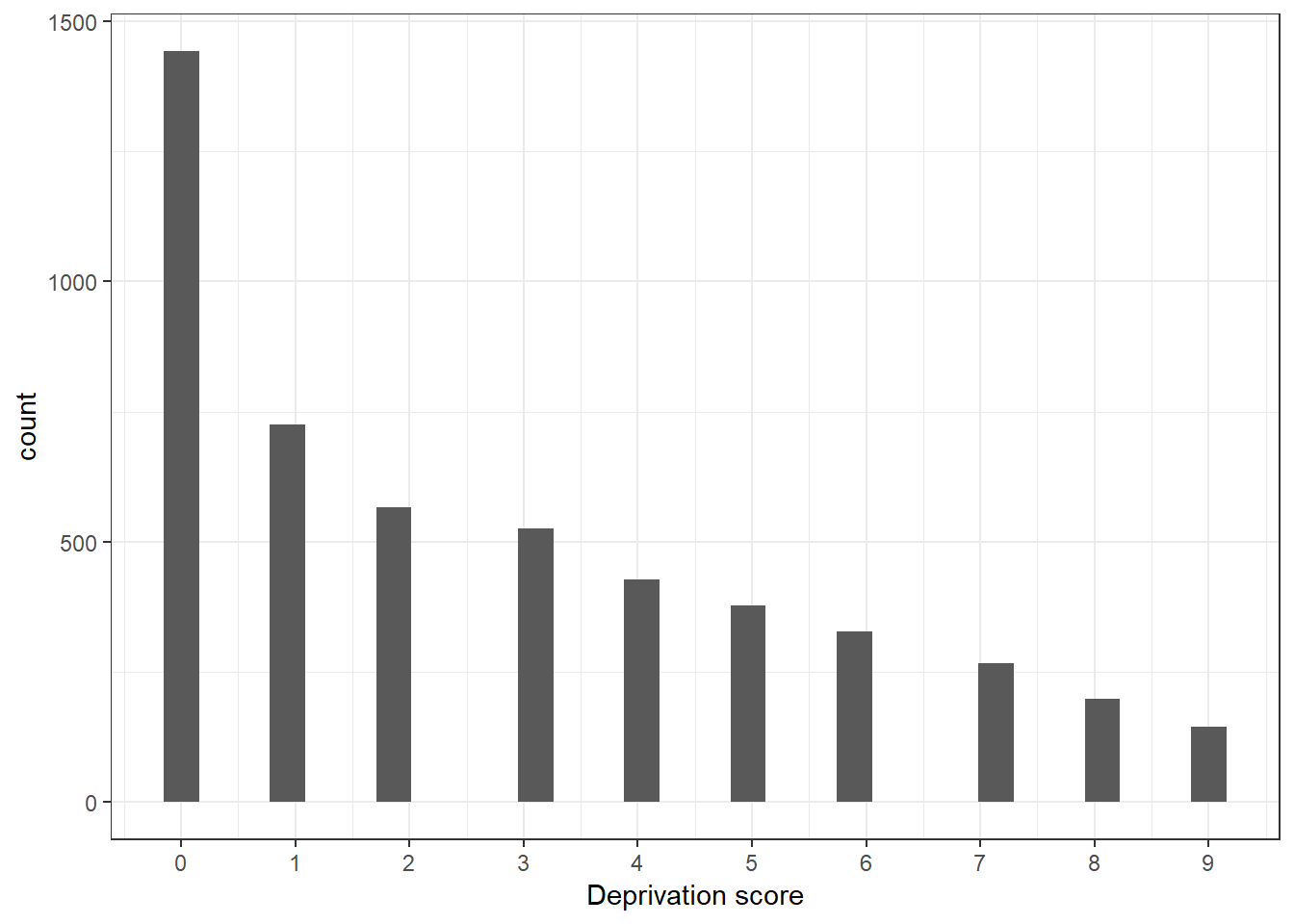

Figure 3.1: This is the histogram of the deprivation score. It shows the number of people by the equally weighted deprivation count.

We see that our deprivation score looks inflated in the right and deflated on the left. This is the expected distribution of a deprivation score in that the majority of the population tends to lack fewer items. This could look very different in very poor countries where most of the population like the majority of basic needs.

To see the relationship between reliability and different scores, we will compute five more scores using different combinations of items. We will see if reliability is affected by the number of items. The correlation matrix shows that if we keep reliable items only, we will have very high correlation with the perfect measure, which in this case is the measure with the nine items (ds). However, we see that, the measure with unreliable items leads to a drop of .93. This is not too bad as \(\omega\) remains high for this scale, but if we drop a couple of items we would see a major drop (.87) (see ds_unrel2).

Rel_MD_1$ds_r2<-rowSums(Rel_MD_1[,c(3:9)])
Rel_MD_1$ds_r3<-rowSums(Rel_MD_1[,c(1,2,4,5,7,8)])
Rel_MD_1$ds_r4<-rowSums(Rel_MD_1[,c(2,3,5,6,8,9)])
Rel_MD_1$ds_r5<-rowSums(Rel_MD_1[,c(1,3,4,6,7,9)])
Rel_MD_1$ds_ur<-rowSums(Rel_MD_1[,c(3:9,10,11)])
Rel_MD_1$ds_ur2<-rowSums(Rel_MD_1[,c(3:7,10,11)])

ds.m<-(Rel_MD_1[,c(17:23)])
ds.cor<-cor(ds.m)
ds.cor

##               ds     ds_r2     ds_r3     ds_r4     ds_r5     ds_ur
## ds     1.0000000 0.9684719 0.9764524 0.9523882 0.9733462 0.9272651
## ds_r2  0.9684719 1.0000000 0.9284786 0.9370200 0.9485305 0.9520979
## ds_r3  0.9764524 0.9284786 1.0000000 0.8875033 0.9371505 0.8899044
## ds_r4  0.9523882 0.9370200 0.8875033 1.0000000 0.8876694 0.8941369
## ds_r5  0.9733462 0.9485305 0.9371505 0.8876694 1.0000000 0.9099612
## ds_ur  0.9272651 0.9520979 0.8899044 0.8941369 0.9099612 1.0000000
## ds_ur2 0.8700863 0.8860309 0.8437632 0.8124119 0.8690256 0.9628708
##           ds_ur2
## ds     0.8700863
## ds_r2  0.8860309
## ds_r3  0.8437632
## ds_r4  0.8124119
## ds_r5  0.8690256
## ds_ur  0.9628708
## ds_ur2 1.0000000

3.5.3 Model-based estimation of overall reliability

The ideal workflow in poverty measurement must include a clear specification of a measurement model. In both the theoretical and applied literature, different authors propose models that suggest that poverty is multidimensional and hierarchical (See Section 1.2). Therefore, in multidimensional poverty measurement we will be almost always interested in assessing reliability using an a priori model and thus we will require to estimate both overall and hierarchical omega (\(\omega\) and \(\omega_h\)). These two can be estimated from an EFA using the R-package psych. However, this book aims to encourage poverty researchers to walk toward the production and assessment of theoretical models, rather than systematically inferring the structure from the data.

This section thus focuses on the examination of reliability when researchers have an a priori measurement model of poverty. Unlike the previous section, the following examples rely on Confirmatory Factor Analysis (CFA) (Brown, 2006). The key difference between an EFA and a CFA is that the second rely on a theoretical model that states the structure of a measure, i.e. a blueprint for measuring poverty (See Section 2.8). A CFA model will examine the extent to which the theoretical model (i.e. number of dimensions, contents of dimensions-indicators, independence of dimensions) manages to reproduce the observed data. In statistical terms, researchers provide a predefined pattern-loading specification. This is specified in equations (2.2) and (2.3). This is just the mathematical formulation of the diagrams shown in section 2.8.

\[\begin{equation} x_{ij} = \lambda_{ij} \eta_j + \varepsilon_ij \end{equation}\]

\[\begin{equation} \eta_j = \gamma_{j} \zeta + \xi \end{equation}\]

Reliability is estimated after a CFA model because both \(\omega\) and \(\omega_h\) rely on two key pieces of information of a CFA model: The factor loadings and the errors. That is, item-factor loadings and the residuals of the model are the key parameters for the estimation of both reliability statistics (See equation (3.6)).

In the following we will show how in both Mplus and R is possible to estimate \(\omega\) and \(\omega_h\). We will start with R and for this purpose we need the lavaan package (Rosseel, 2012). This package comprises a series of functions to estimate different kinds of latent variable models such as measurement and analytic models like Structural Equation Models (SEM). Once the CFA model is fitted with the R-package lavaan, the function omegaFromSem() of the psych R-package can be used to estimate \(\omega\) and \(\omega_h\). However, we will show how this can be done by hand to gain insight of the differences between the two reliability statistics and to operationalise the process using the Mplus estimates.

3.5.3.1 Computation using R

We will continue using our simulated data (“Rel_MD_data_1_1.dat”). As a remainder we have stored the data on the object Rel_MD_1 (see above). So the first question we need to answer is What is the structure of our measure?. That is, how many dimensions and how many indicators (and which indicators) for each dimension. In this case, we will assume that our theory tells us that we have a higher-order factor (poverty), three subfactors (dimensions of poverty) and three indicators for each dimension. With that in mind, we need to tell lavaan how our model looks like and, because \(\omega\) and \(\omega_h\) is easier to compute from Schmid & Leiman (1957) transformation, we will specify such type of model directly rather than a nested model. To do so, we will store the model on the object MD_model. We are saying something very simple. First, we are saying that the higher-order factor h has nine manifest variables (x1-x9). Then we say that each dimension has three outcome variables. For example, F1 has x7, x8 and x9. Then we tell lavaan that our factor variance are equal to zero for identification and being consistent with the Schmid & Leiman (1957) transformation.

#Omega from Sem
library(lavaan)
# We first specify the model
MD_model <- ' h =~ +x1+x2+x3+x4+x5+x6+x7+x8+x9 
                F1=~  + x7 + x8 + x9        
                F2=~  + x4 + x5 + x6         
                F3=~  + x1 + x2 + x3
                h  ~~ 0*F1
                h  ~~ 0*F2
                h  ~~ 0*F3
                F1 ~~ 0*F2
                F2 ~~ 0*F3
                F1 ~~ 0*F3

'

Once we have specified our model, we can proceed to tell lavaan to estimate the model. To fit the CFA model we will use sem function which has been harmonised with the functions cfa and lavaan. Remember that the kind of variables we have are categorical -so we include the option ordered() and we will request standardised loadings with std.lv=TRUE. We will store the output on the object fit.

fit <- sem(MD_model, data = Rel_MD_1, 
           ordered=c("x1","x2","x3","x4","x5",
                     "x6","x7","x8","x9"),
           std.lv=TRUE)
# The command below is to check the output (We will check this in the 
#next section and validity chapter)
#summary(fit, fit.measures=TRUE, rsquare=TRUE, standardized=TRUE)

Before showing the authomated way to estimate \(\omega\) and \(\omega_h\), we will show the manual computation. There are two main parameters one needs for their computation: factor loadings from the indicators to the overall factor (\(\lambda_h\)), to each dimension (\(\lambda_j\)) and the error. This can be easily extracted from the fit object as follows:

lambdas<-as.data.frame(fit@Model@GLIST$lambda)
error<-colSums(fit@Model@GLIST$theta)

The then the square of the sum of the loadings (\(\lambda_h\)) and (\(\lambda_j\)) is taken as well as the sum of the error. The we can compute both \(\omega\) and \(\omega_h\) using equation (3.6) and (3.7).

Slambda_2<-sum(lambdas[1])^2 + sum(lambdas[2])^2 + 
           sum(lambdas[3])^2 + sum(lambdas[4])^2
error <- sum(error)

omega_t <- Slambda_2 / (Slambda_2+error)
omega_h <- sum(lambdas[1])^2 / (Slambda_2+error)
omegamanual<-c(omega_h=omega_h,omega_t=omega_t)
omegamanual

##   omega_h   omega_t 
## 0.8445022 0.9707344

Fortunately, there is an R function from the psych package that does this for us. Once the model has been fitted, we apply the function omegaFromSem() to request the estimates and store the estimates of both \(\omega\) and \(\omega_h\) in the omegasem object. The results indicate high overall reliability and high reliability after considering the multidimensional features of the scale.

omegasem<-omegaFromSem(fit)
omegasem<-c(omega_h=omegasem$omega,
            omega_t=omegasem$omega.tot)
omegasem

##   omega_h   omega_t 
## 0.8446990 0.9707276

3.5.3.2 Computation using Mplus via R

The R-package mplusAutomation is an excellent alternative to automate Mplus from within R -so you get track of your input files and do not get lost with so many windows- (Hallquist & Wiley, 2018). We can create within R an Mplus object as follows using the function mplusObject(). The syntax is the standard Mplus syntax to fit a model. What we need to tell Mplus is the name of the variables, the type of variables and which variables is going to use. Then in the ANALYSIS section, we instruct Mplus to use the wlsmv estimator and four cores⁸. Then we tell Mplus that the overall factor h has nine outcome measures and that each dimension has three indicators. We set the variances equal to zero to be consisten with the Schmid & Leiman (1957) transformation. As with lavaan we will fit a bi-factor model. We will store the syntax in the object test.

test <- mplusObject(
TITLE = "Bi-factor model CFA;",
   VARIABLE = "
     NAMES = x1-x11 resources educ_yr occupation class;
     CATEGORICAL = x1-x9;
     USEVARIABLES = x1-x9;",
   ANALYSIS = "ESTIMATOR = wlsmv;
              PROCESS = 4;",

MODEL = "f1 by x1-x3;
  f2 by x4-x6;
  f3 by x7-x9;
  h by x1 x2 x3 x4 x4 x5 x6 x7 x8 x9;
  F1 with F2@0;
  F2 with F3@0;
  F3 with F1@0;
  h with f1@0;
  h with f2@0;
  h with f3@0;",

OUTPUT = "std stdyx;")

Now we have the model specyfication saved on the test object. We need know to pass this R syntax to Mplus (*.inp). The function mplusModeler() is going to do this for us. We tell the function that we have the object test, that we want an Mplus syntax file named “rel_CFA_2.inp”, and to tell Mplus to use the following data “Rel_MD_data_1_1.dat”. This function permits estimating the model directly using the option run⁹

res <- mplusModeler(test, modelout = "rel_CFA_2.inp", 
                    writeData = "never", hashfilename = FALSE, 
                    dataout="Rel_MD_data_1_1.dat", run = 1L)

## 
## Running model: rel_CFA_2.inp 
## System command: C:\WINDOWS\system32\cmd.exe /c cd "." && "Mplus" "rel_CFA_2.inp" 
## Reading model:  rel_CFA_2.out

Once the model has been run, we can import the output using the function readModels(). We will explore the full output in the next chapter as for now we will focus in the estimation of \(\omega\) and \(\omega_h\). The factor loadings of the Bi-factor model are stored on a R list (parameters). We request the standardised estimates as we did with lavaan. We can also ask for the error from the `r2 object in the parameters list. Once we have the parameters, we can proceed as above to estimate the reliability statistics. We see that we could replicate the results from lavaan.

REL_CFA_2<-readModels(filefilter ="rel_CFA_2")

## Reading model:  C:/Proyectos Investigacion/PM Book/rel_cfa_2.out

lambdas<-REL_CFA_2$parameters$std.standardized[1:18,1:3]
error<-REL_CFA_2$parameters$r2[6]

lambda_2<-sum(lambdas[10:18,3])^2 + sum(lambdas[1:3,3])^2 + 
          sum(lambdas[4:6,3])^2 + sum(lambdas[7:9,3])^2
error <- sum(error)

omega_t <- lambda_2 / (lambda_2+error)
omega_h <- sum(lambdas[10:18,3])^2 / (lambda_2+error)

omega_t

## [1] 0.9707333

omega_h

## [1] 0.8445348

3.5.4 Overall reliability and population orderings

One of the predictions of measurement theory is that reliability leads to consistent population orderings, i.e. poor people will have high deprivation scores and not poor people will have low deprivation scores (see Table (3.2). We have illustrated this point using the correlation between the different deprivation scores corresponding to diverse levels of overall reliabilities. We can follow up that example by looking at the values of the latent variable for the multidimensional reliable measure (Rel_MD_1). After fitting the CFA model we just can simply use the function predict() to obtain the Maximum Likelihood estimates of the latent variable. Then we can merge these values with our data set. The prediction will generate four estimates for the latent variables. The overall factor (h) and the values for the three dimensions.

factor_scores<-predict(fit)
Rel_MD_1<-cbind(Rel_MD_1,factor_scores)
head(Rel_MD_1[,c(21:24)])

##   ds_r5 ds_ur ds_ur2          h
## 1     3     2      2  0.4475885
## 2     0     0      0 -0.6781638
## 3     1     1      1 -0.2440620
## 4     2     1      1  0.2851351
## 5     1     2      2 -0.2207057
## 6     1     0      0 -0.2207057

To contrast the values of the reliable multidimensional measure with the values of a slightly less reliable measure we will fit a new model. As in the previous example (Section @ref(#Chapter-3-expoverel)), we will replace the first two indicators x1 and x2 by x10 and x11. Both load into the first factor (f1). The estimates are stored in a different object (fit_ur) and estimate the factor scores using the predict() function. Finally, we inspect the values.

## We first specify the model
MD_model <- ' h =~ +x10+x11+x3+x4+x5+x6+x7+x8+x9 
                F1=~  + x7 + x8 + x9        
                F2=~  + x4 + x5 + x6         
                F3=~  + x10 + x11 + x3
                h  ~~ 0*F1
                h  ~~ 0*F2
                h  ~~ 0*F3
                F1 ~~ 0*F2
                F2 ~~ 0*F3
                F1 ~~ 0*F3

'

fit_ur <- sem(MD_model, data = Rel_MD_1, 
           ordered=c("x10","x11","x3","x4","x5","x6","x7","x8","x9"),
           std.lv=TRUE)
factor_scores_ur<-predict(fit_ur)
colnames(factor_scores_ur)[1:4]<-c("hur","F1ur","F2ur","F3ur")
Rel_MD_1<-cbind(Rel_MD_1,factor_scores_ur)
head(Rel_MD_1[,c(25:28)])

##            F1         F2         F3         hur
## 1 -0.81293477 -0.1296229  1.2478407  0.38436469
## 2 -0.08627376 -0.1536510 -0.1720003 -0.59656764
## 3 -0.28822588  0.5290560 -0.3986557 -0.10512455
## 4  0.13806885 -0.7559100  0.7442695 -0.05228111
## 5 -0.30252106 -0.3910445  0.4514504 -0.50856087
## 6 -0.30252106 -0.3910445  0.4514504 -0.59656764

To assess the consistency of both multidimensional scales we will plot the latent factor values by the deprivation score. Figure 3.2 shows that the factor scores are very similar within each deprivation group. For each deprivation score we find very different factor scores, indicating that the deprivation scores is a good measure to rank and split the population according to the severity of deprivation. In contrast, figure 3.3 show that although there is relationship between the deprivation score and factor scores, this relationship is more noisy. Not only there is much more variability within each deprivation group but also there is some overlap. That means that if we use some cut off to split the poor from the not poor based on a deprivation score, we will be more likely to confound both groups. In this case, the mixing of groups is not that dramatic as the scale is still somewhat reliable, but it could be very noisy for less reliable scales.

require(ggplot2)
g <- ggplot(Rel_MD_1, aes(as.factor(ds), h))
g + geom_boxplot(varwidth=T) + 
    labs(x="Deprivation score. Reliable",
         y="Factor score (Latent variable)") + theme_bw()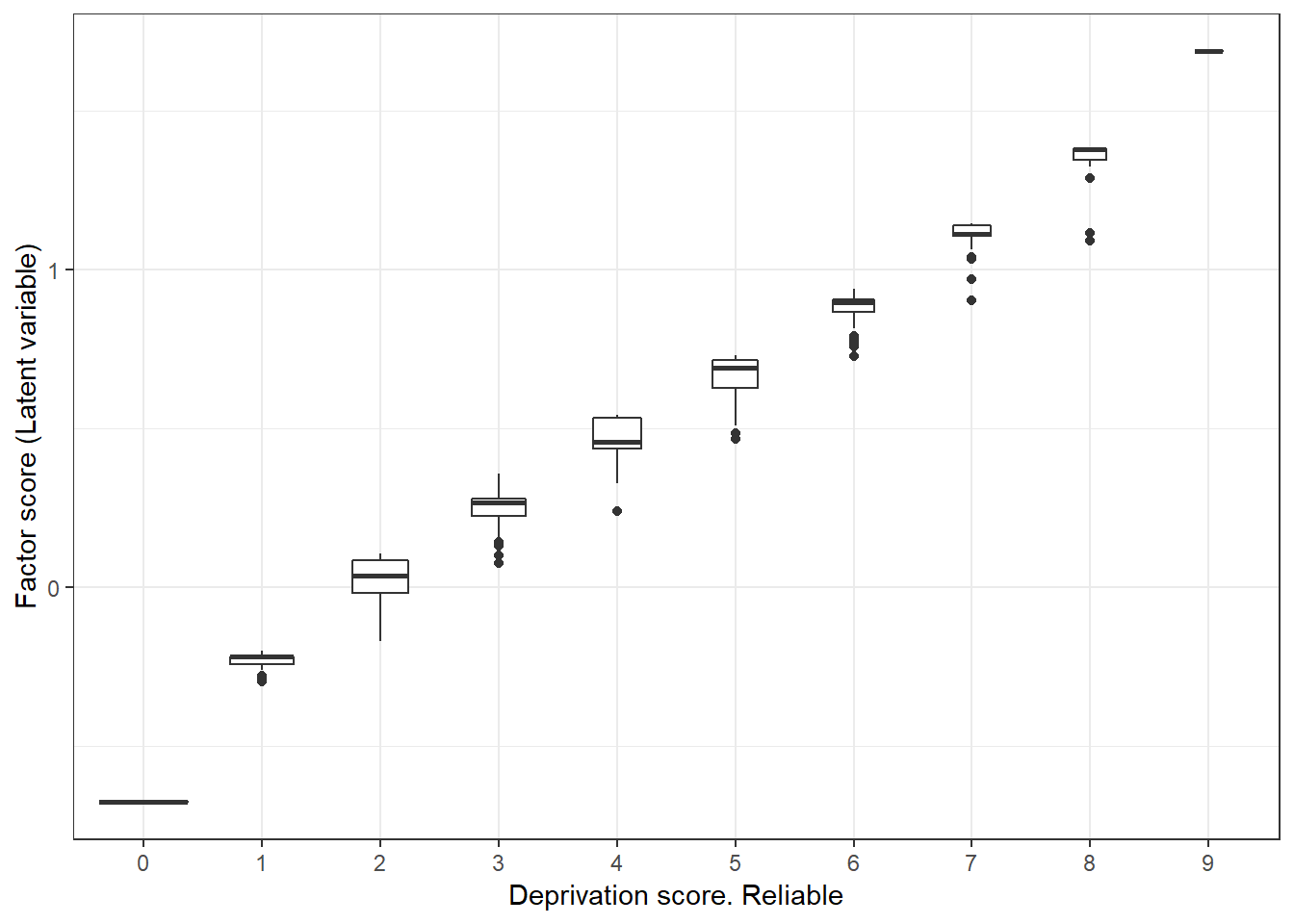

Figure 3.2: Relationship between the deprivation score (x1-x9) and the latent variable score. We appreciate the narrowness of the box plots, indicating good group separation.

g <- ggplot(Rel_MD_1, aes(as.factor(ds_ur), hur))
g + geom_boxplot(varwidth=T) + 
    labs(x="Deprivation score. Unreliable",
         y="Factor score (Latent variable)") + theme_bw()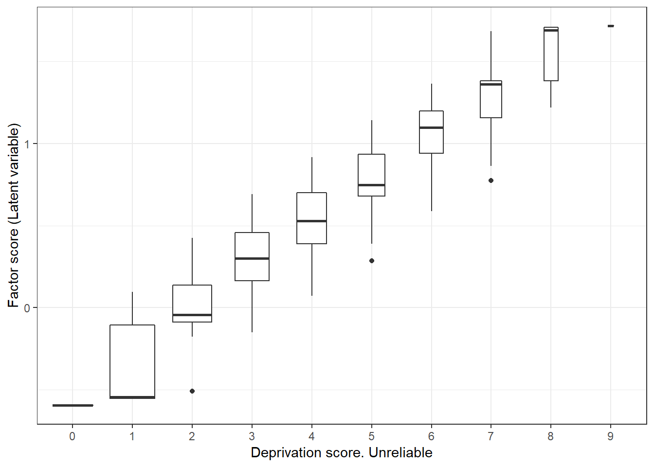

Figure 3.3: Relationship between the deprivation score (x10, x11 and x3-x9) and the latent variable score. There is more variability in this case indicating poor group separation.

3.5.5 Item-level reliability

3.5.5.1 Estimation with R

Overall reliability is an excellent summary of the quality of an index in that it tells the homogeneity of our scale and its capacity to produce consistent population rankings. In section @ref(#relestimation) we showed that including some uncorrelated items lead to a reduction of reliability and that this has negative implication for consistency across measurements. This section focuses on item reliability, i.e. how specific items contribute positively or negatively to reliability.

Section 3.4 reviewed Item Response Theory (IRT), which is a theory of the properties of indicators by putting forward the concepts of discrimination and severity. The standard IRT modelling assumes that scales are unidimensional in that indicators are manifest of a latent trait. However, in parallel to the development of CFA, IRT modelling has incorporated multidimensional models. However, as long as a scale is homogeneous, the bias from a multidimensional IRT and the unidimensional one should not dramatically change our conclusions about the reliability of the items.

To illustrate IRT modelling, we will work with the same data set, which we know that results in a highly homogeneous scale. We will use the data “Rel_MD_1” and the R-package ltm which fits different kinds of IRT models. The ltm() function fits one, two and three-parameter IRT models. Below we fit a two-parameter IRT model simply by adding the z1 option so we allow the model to have different slopes, i.e. Two-parameter IRT model. The output shows the difficulty and discrimination coefficients. The difficulty represents the severity of the deprivation on the latent trait. For example, item x1 is less severe than item x3. The second column Dscrmn displays the values of the discrimination parameters. All the items have values \(>.9\) which is above the suggested threshold by Guio et al. (2016) and Nájera (2018).

library(ltm)
rel_irt<-ltm(Rel_MD_1[,c(1:9)] ~ z1)
rel_irt

## 
## Call:
## ltm(formula = Rel_MD_1[, c(1:9)] ~ z1)
## 
## Coefficients:
##     Dffclt  Dscrmn
## x1   0.023   2.290
## x2   0.702   2.183
## x3   1.258   2.198
## x4   0.053   2.306
## x5   0.698   2.368
## x6   1.297   2.154
## x7   0.160   2.541
## x8   0.802   2.547
## x9   1.236   2.477
## 
## Log.Lik: -20132.92

Before checking the estimation with Mplus, we will check what will happen if we include our unreliable items. Items x1 and x2 are replaced by items V1 and V2. As expected, the discrimination values are unacceptably low as well as the severity values which are (\(\geq3\)) standard deviations.

head(Rel_MD_1[,c(3:11)])

##   x3 x4 x5 x6 x7 x8 x9 x10 x11
## 1  1  1  0  0  0  0  0   0   0
## 2  0  0  0  0  0  0  0   0   0
## 3  0  1  0  0  0  0  0   0   0
## 4  0  0  0  0  1  0  0   0   0
## 5  0  0  0  0  0  0  0   1   1
## 6  0  0  0  0  0  0  0   0   0

rel_irt_2<-ltm(Rel_MD_1[,c(3:11)] ~ z1)
rel_irt_2

## 
## Call:
## ltm(formula = Rel_MD_1[, c(3:11)] ~ z1)
## 
## Coefficients:
##      Dffclt  Dscrmn
## x3    1.426   1.651
## x4    0.053   2.371
## x5    0.689   2.488
## x6    1.279   2.245
## x7    0.157   2.817
## x8    0.780   2.840
## x9    1.193   2.804
## x10   5.142   0.133
## x11   4.882   0.135
## 
## Log.Lik: -21740.2

3.5.5.2 Mplus estimation within R

Similarly we can fit the model using items (x1-x9) in Mplus using the package “mplusAutomation” by creating an object with mplusObject().

test <- mplusObject(
TITLE = "IRT model;",
   VARIABLE = "
     NAMES = x1-x9 resources educ_yr occupation hh_size class;
     CATEGORICAL = x1-x9;
     USEVARIABLES = x1-x9;",
   ANALYSIS = "ESTIMATOR = ml;
              PROCESS = 4;",

MODEL = "h by x1* x2-x9;
         h@1;")

Then the model is fitted using mplusModeler(). We will name our Mplus script as “rel_IRT_1.inp” and we will be using the same data as before (“Rel_MD_data_1_1.dat”) and we request Mplus to run the model directly from the script with (run).

res <- mplusModeler(test, modelout = "rel_IRT_1.inp", 
                    writeData = "never", hashfilename = FALSE, 
                    dataout="Rel_MD_data_1_1.dat", run = 1L)

Now we read the result of our model with readModels().

REL_IRT_1<-readModels(filefilter ="rel_IRT_1")

The readModels() does an excellent job in extracting and ordering the Mplus output. It puts all the relevant result in lists. We can see that the Mplus estimates are very similar to those obtained from the ltm package.

rel_irt<-REL_IRT_1$parameters$irt.parameterization
rel_irt<-rel_irt[1:18,]
rel_irt<-data.frame(a=rel_irt$est[1:9],b=rel_irt$est[10:18])
rel_irt

##       a     b
## 1 2.290 0.024
## 2 2.192 0.700
## 3 2.207 1.254
## 4 2.312 0.054
## 5 2.383 0.696
## 6 2.172 1.291
## 7 2.548 0.161
## 8 2.561 0.800
## 9 2.498 1.231

3.6 Multidimensional item-reliability evaluation

A multidimensional IRT model is just a CFA model with categorical indicators. One way to assess the item-level reliability is by looking at the loadings from a CFA model. We can fit a higher-order factor model (equivalent to the bi-factor model above) to assess the value of the loadings and and look at the \(R^2\) values of each indicator (which is just \(\lambda{hj}^2\)). \(R^2\leq.25\) are equivalent to \(\lambda{hj}^2\leq.5\), which are often used as cut offs of unacceptably low loadings. We see that all these items are highly reliable not only with regard the higher order factor but also in terms of each dimension, measured by each factor loading.

 MD_model <- ' f1  =~ x1 + x2 + x3
              f2 =~ x4 + x5 + x6
              f3   =~ x7 + x8 + x9
                h =~ f1 + f2 + f3
 '

fit <- sem(MD_model, data = Rel_MD_1,
           ordered=c("x1","x2","x3","x4","x5",
                     "x6","x7","x8","x9"))
inspect(fit,what="std")$lambda

##       f1    f2    f3 h
## x1 0.924 0.000 0.000 0
## x2 0.888 0.000 0.000 0
## x3 0.873 0.000 0.000 0
## x4 0.000 0.929 0.000 0
## x5 0.000 0.917 0.000 0
## x6 0.000 0.866 0.000 0
## x7 0.000 0.000 0.947 0
## x8 0.000 0.000 0.916 0
## x9 0.000 0.000 0.894 0

3.6.1 Item-reliability and monotonicity

Low loadings are an indication that the indicator is not a manifest variable of the underlying construct. That is, that changes in poverty do not mirror changes in deprivation. Section 3.4 suggested that there is a relationship between item-reliability and the monotonicity axiom. Nájera (n.d.) shows that indeed low loadings approximately \(\leq.5\) lead to violations of the strong monotonicity axiom, i.e. a reduction in poverty does not reflect an improvement in the achievement matrix. Weak monotonicity is violated when an improvement in poverty results in an increase of deprivation, this would happen when the factor loadings are negative, for example.

We will fit a higher order model using again the unreliable items (x10 and x11) instead of x1 and x2. Of course, it is possible to use either the loadings of the \(R^2\) values (these can be obtained with the summary() function. We see again, as in the IRT analysis that both items have unacceptably low values. These items should be dropped from the scale as it inclusion introduces noise to our measure. That would imply dropping the first dimension in the absence of alternative indicators.

 MD_model <- ' f1  =~ x10 + x11 + x3
              f2 =~ x4 + x5 + x6
              f3   =~ x7 + x8 + x9
                h =~ f1 + f2 + f3
 '

fit <- sem(MD_model, data = Rel_MD_1,
           ordered=c("x10","x11","x3","x4","x5",
                      "x6","x7","x8","x9"))

## Warning in lav_object_post_check(object): lavaan WARNING: some estimated ov
## variances are negative

inspect(fit,what="std")$lambda

##        f1    f2    f3 h
## x10 0.114 0.000 0.000 0
## x11 0.116 0.000 0.000 0
## x3  1.036 0.000 0.000 0
## x4  0.000 0.924 0.000 0
## x5  0.000 0.920 0.000 0
## x6  0.000 0.868 0.000 0
## x7  0.000 0.000 0.947 0
## x8  0.000 0.000 0.914 0
## x9  0.000 0.000 0.898 0

3.7 Real data example

We will use the Mexican data set “Mex_pobreza_14.dat”. This data set contains a subset of the deprivation indicators utilised to measure multidimensional poverty in Mexico. The official measure has two domains: income and social rights. The social rights domain has five dimensions: essential services, housing, food deprivation, social security and education. Some of this dimensions are measured with few indicators, like education and social security. This poses limitations to fit an identified model. Hence, we will use a reduced version of the model comprising three dimensions: essential services, housing and food deprivation.

The Mexican poverty data comes from a nationally representative complex survey. We will use the package “survey” (Lumley, 2016). This is a comprehensive R-package to analyse survey data. We strongly advice readers to check Lumley (2011) book on complex surveys to get a depth insight on complex sampling and the use of Lumley’s excellent package. To produce design deprivation rates estimates for each of the 14 items we need to specify few things. First, we need to identify the sampling weights and the primary sampling units (PSU). The options(scipen=999, survey.lonely.psu="adjust") instruction is to prevent errors as sometimes there is one household per PSU. Once we have set up the sampling design we can estimate the deprivation rates with the svymean() function -we have rounded the percentages for simplicity; never try to be too accurate with survey data-. We can see than deprivation in the housing dimension items is rather low. Essential services present higher deprivation rates but electricity is very low. We see that the food deprivation items have the higher rates on average.

library(haven)
Mex_D<-read_dta("pobreza_14.dta")

cols <- c("icv_muros", "icv_techos", "icv_pisos", "icv_hac",
          "isb_agua","isb_dren", "isb_luz", "isb_combus",
          "ic_sbv", "ia_1ad", "ia_2ad", "ia_3ad", "ia_4ad", 
          "ia_5ad",  "ia_6ad")

library(survey)
options(scipen=999, survey.lonely.psu="adjust")
des <- svydesign(data=Mex_D, id=~1, CLUSTER=~psu, weights=~weight)
propr <- data.frame(svymean(Mex_D[, cols],des,na.rm=T))
propr <- round(propr*100,1)
propr

##            mean  SE
## icv_muros   1.7 0.1
## icv_techos  1.6 0.1
## icv_pisos   3.0 0.1
## icv_hac     5.6 0.1
## isb_agua    7.7 0.1
## isb_dren    7.5 0.1
## isb_luz     0.8 0.0
## isb_combus 12.0 0.2
## ic_sbv     19.6 0.2
## ia_1ad     33.3 0.3
## ia_2ad     15.9 0.2
## ia_3ad     24.9 0.2
## ia_4ad     14.0 0.2
## ia_5ad     16.4 0.2
## ia_6ad     12.3 0.2

3.7.1 Overall reliability

Now the we are familiarised with the 14 deprivation indicators we can proceed to estimate the reliability statistics. We will fit the model in Mplus as we will incorporate the survey design in the estimation of the parameters -it is possible to do so with the lavaan.survey() too-. We first create our Mplus script (rel_CFA_mex.inp) to fit the bi-factor model. Following the theoretical model for this data, the model has three dimensions (housing (f1), essential services (f2) and food deprivation (f3)) and one higher-order factor (h). Once the model has been fitted we will store the output in the object called REL\_CFA\_mex.

test <- mplusObject(
TITLE = "Bi-factor model CFA;",
   VARIABLE = "
     NAMES = proyecto folioviv foliohog icv_muros icv_techos 
             icv_pisos icv_hac isb_agua isb_dren isb_luz isb_combus
             ic_sbv ia_1ad ia_2ad ia_3ad ia_4ad ia_5ad ia_6ad
             ia_7men ia_8men ia_9men ia_10men ia_11men ia_12men 
             tv_dep radio_dep fridge_dep
             washingmach_dep compu_dep inter_dep psu weight
             rururb tot_integ durables educ_hh; 
MISSING=.;
     CATEGORICAL = icv_muros icv_techos icv_pisos icv_hac isb_agua
                   isb_dren isb_luz isb_combus  ia_1ad 
                   ia_2ad ia_3ad ia_4ad ia_5ad ia_6ad;
     USEVARIABLES = icv_muros icv_techos icv_pisos icv_hac isb_agua
                   isb_dren isb_luz isb_combus  ia_1ad 
                   ia_2ad ia_3ad ia_4ad ia_5ad ia_6ad;

WEIGHT=weight;
cluster = psu;",

   ANALYSIS = "TYPE = complex;

ESTIMATOR = wlsmv;
PROCESS = 4;",

MODEL = "f1 by icv_muros icv_techos icv_pisos icv_hac;
  f2 by isb_agua
        isb_dren isb_luz isb_combus;
  f3 by ia_1ad ia_2ad ia_3ad ia_4ad ia_5ad ia_6ad;
  h  by icv_muros icv_techos icv_pisos icv_hac isb_agua
        isb_dren isb_luz isb_combus ia_1ad ia_2ad 
        ia_3ad ia_4ad ia_5ad ia_6ad;
  F1 with F2@0;
  F2 with F3@0;
  F3 with F1@0;
  h with f1@0;
  h with f2@0;
  h with f3@0;",

OUTPUT = "std stdyx;")

mplusModeler(test, modelout = "rel_CFA_mex.inp", 
                    writeData = "never", hashfilename = FALSE, 
                    dataout="Mex_pobreza_14.dat", run = 1L)
REL_CFA_mex<-readModels("rel_CFA_mex.out")

We then can estimate the overall reliability statistics; both \(\omega\) and \(\omega_h\)¹⁰. The reliability of our measure is very high under both statistics and both are above the recommended thresholds (Nájera, 2018). To estimate the reliability measures we will use the same approach we followed in the previous section. First, we will obtain the factor loadings (f’s and h) and the errors for each indicator. Then we will take the square of the sum of the lambdas (f1, f2, f3 and h) and the error sum. \(\omega\) and \(\omega_h\) then can be calculated using formulas from equations (3.6) and (3.7).

The values of both \(\omega\) and \(\omega_h\) are high .97 and .81, respectively. These figures suggest that this multidimensional scale is homogeneous but has multidimensional features (\(\omega_h<\omega\)).

lambdas<-REL_CFA_mex$parameters$std.standardized[1:28,1:3]
error<-REL_CFA_mex$parameters$r2[6]

lambda_2<-sum(lambdas[10:28,3])^2 + sum(lambdas[1:4,3])^2 + 
          sum(lambdas[5:8,3])^2 + sum(lambdas[9:14,3])^2
error <- sum(error)

omega_t <- lambda_2 / (lambda_2+error)
omega_h <- sum(lambdas[10:28,3])^2 / (lambda_2+error)

omega_t

## [1] 0.9730641

omega_h

## [1] 0.8058398

3.7.2 Item-level reliability

Once we have assessed the overall reliability of the Mexican index, we can assess item-reliability by fitting a higher-order factor model and checking the value of the factor loadings. We just simply need to rewrite our model (rel_CFA_mex2.inp) to represent a structure where the dimensions load into the higher order factor (i.e. we will not fit a bi-factor model but a hierarchical factor model). This is simply done by specifying that the higher-order factor h is measured by the three dimensions (f1, f2 and f3) and each dimension has several indicators.

test <- mplusObject(
TITLE = "CFA higher order model CFA;",
   VARIABLE = "
     NAMES = proyecto folioviv foliohog icv_muros icv_techos 
             icv_pisos icv_hac isb_agua isb_dren isb_luz isb_combus
             ic_sbv ia_1ad ia_2ad ia_3ad ia_4ad ia_5ad ia_6ad
             ia_7men ia_8men ia_9men ia_10men ia_11men ia_12men 
             tv_dep radio_dep fridge_dep
             washingmach_dep compu_dep inter_dep psu weight
            rururb tot_integ; 
MISSING=.;
     CATEGORICAL = icv_muros icv_techos icv_pisos icv_hac isb_agua
                   isb_dren isb_luz isb_combus  ia_1ad 
                   ia_2ad ia_3ad ia_4ad ia_5ad ia_6ad;
     USEVARIABLES = icv_muros icv_techos icv_pisos icv_hac isb_agua
                   isb_dren isb_luz isb_combus  ia_1ad 
                   ia_2ad ia_3ad ia_4ad ia_5ad ia_6ad;

WEIGHT=weight;
cluster = psu;",

   ANALYSIS = "TYPE = complex;

ESTIMATOR = wlsmv;
PROCESS = 4;",

MODEL = "f1 by icv_muros icv_techos icv_pisos icv_hac;
  f2 by isb_agua
        isb_dren isb_luz isb_combus;
  f3 by ia_1ad ia_2ad ia_3ad ia_4ad ia_5ad ia_6ad;
  h by f1 f2 f3;",

OUTPUT = "std stdyx;")

mplusModeler(test, modelout = "rel_CFA_mex2.inp", 
                    writeData = "never", hashfilename = FALSE, 
                    dataout="Mex_pobreza_14.dat", run = 1L)

We can request the standardised factor loadings and inspect its values using the readModels() function. To facilitate our interpretation we can plot the standardised loadings (Figure 3.4. We see that all the indicators have very high loadings and above the suggested threshold (\(\lambda_ij>.5\)). That means that these indicators discriminate well and are reliable manifests of each dimension. We see, nonetheless, that the indicators of the housing dimension tend to have low values. This could be an indication that these indicators are losing discriminatory power due to changes in living standards and that the Mexican measure might need some updating.

REL_CFA_mex2<-readModels("rel_CFA_mex2.out")
modelParams<- REL_CFA_mex2$parameters$std.standardized[1:14,]
modelParams <- subset(modelParams, select=c("paramHeader", "param", "est", "se"))

library(ggplot2)
limits <- aes(ymax = est + se, ymin=est - se)
 ggplot(modelParams, aes(x=param, y=est)) + geom_pointrange(limits) +scale_x_discrete("") +
   geom_hline(yintercept=0, color="grey50") + theme_bw() +ylab("Std Loading") + coord_flip()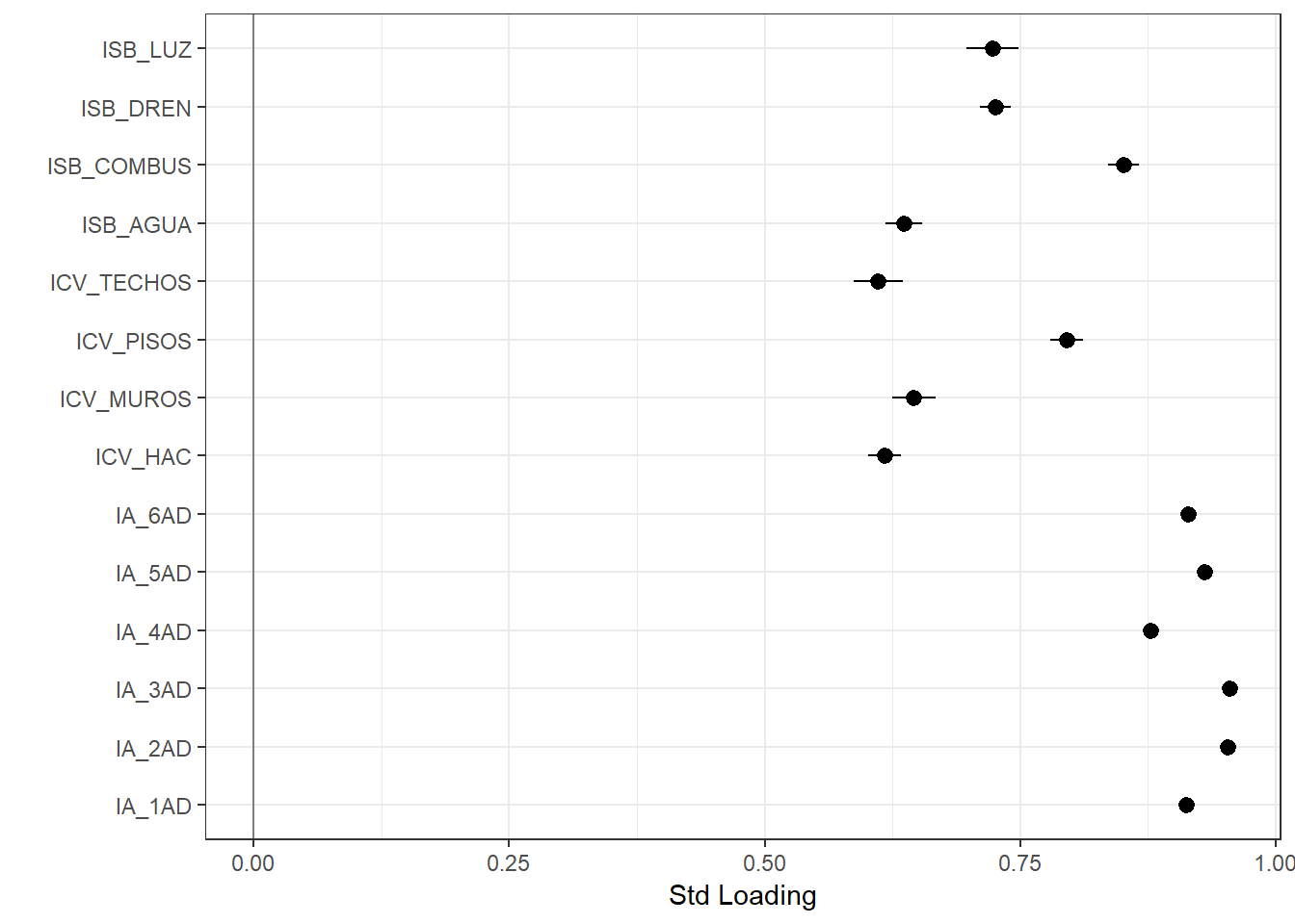

Figure 3.4: This plot shows the standardised values of the loadings for the 14 items.

#Final comments

We have reviewed the theory, implementation and both positive and negative implications for measurement of reliability. In social sciences, we tend to work with concepts that are unlikely to be captured by a single variable. Instead, we work on an indirect way. We believe that our concepts produce certain manifestations and we use these outcomes as means to measure our constructs. This process could have very high or very low uncertainty and we would like to reduce it as much as we can. Reliability is a key principle that helps researchers to assess the extent to which they can distinguish signal from noise. In doing so, researchers are also more likely to know whether a set of indicators helps them to produce a ranking of the population. In the case of poverty, from very severe to the mild forms of deprivation.

The assessment of reliability involves acknowledging that in multidimensional poverty measurement we must raise a number of assumptions. Testing reliability help us to examine the extent to which our prejudices introduce noise and to detect which components of our scales need to be reworked.

The presumed nature of poverty (multidimensionality) demands using appropriate methods for its scrutiny. We have put forward \(\omega\) and \(\omega_h\) as the two most adequate statistics to estimate reliability for multidimensional scales. At this point, we have shown that a reliable measure will result in adequate population rankings, but this is not enough. So far, we know whether our indicators produce consistent results but we know little about whether the indicators in question are outcomes of poverty. In other words, we believe that the latent variable is poverty, but we have not checked whether that is the case. The next chapter concerns with the question of hitting the target, i.e. measuring what we want to measure.

---

4. We say latent because at this point we are thinking in terms of reliability and we have not proved that the scale measures living standards and poverty. The Chapter on Validity explains this difference↩

5. In Chapter 1 we underlined the fact that we cannot claim to observe poverty directly as it is an invention of the human mind but we could claim that our theory of poverty tells us what kind of manifestations (in form of deprivation) will inform us about people’s low living standards↩

6. Interestingly enough, this is a desirable property in Sen’s Axiomatic approach in the form of the monotonicity axiom Nájera (n.d.), see 3.4↩

7. If the scale is badly constructed reliability could be negative using some statistics like \(\alpha\)↩

8. The wlsmv estimator uses robust Weighted Least Squares to run the CFA. This estimator is a good approximation, relative to Maximum Likelihood (ML), that is less computationally intensive and feasible when having several factor, we strongly recommend to check the Mplus documentation and Brown (2006) excellent book for further insights↩

9. The reader will appreciate that the file “rel_CFA_2.inp” can be opened in Mplus.↩

10. Prior the estimation of the reliability statistics is vital to inspect the fit of the model as a poor model will not be useful to estimate omega. We will discuss in the next chapter (Validity) the meaning of these statistics. At this point we will focus on the fact that a poor model fit invariably leads to poor estimates of reliability. There is no point in estimating reliability of a scale that makes no sense at all. To assess the fit of the model we look at four statistics: \(\chi^2\), TLI, CFI and RMSEA. For this model the relative statistics of fit look fine and we have some certainties about the model we fit.↩