Chapter 5 Comparability in poverty measurement
Abstract
This chapter discusses the problem of comparability in poverty measurement and frames this challenge using the principle of measurement invariance. The chapter provides an intuitive explanation of measurement invariance. A connection between measurement invariance, validity and reliability is provided. Then the chapter uses simulated data to illustrate how measurement invariance works and how can it be analysed in Mplus. The chapter also provides a real-data example.
5.1 Measurement invariance
Making comparisons of poverty across time or units (countries, regions, population groups) is one of the chief goals in poverty research. Ideally, changes in poverty from a given year to another must reflect effective changes in living standards. The same must hold when comparing estimates across groups where poverty must be relatively higher or lower given differences in living standards across the units of interest. Nonetheless, survey data is subject to different kinds of amendments overtime. There are changes to the questionnaire that aim to update poverty indices, researchers also include or exclude different indicators overtime and across groups, data collection modes and sampling frameworks might differ. These modifications are likely to affect the comparability of poverty estimates overtime or across countries using similar data.
In poverty measurement the literature often proposes that if one has the same indicators, poverty is being measured on equivalent terms. MI transforms this proposition into an assumption as there is no guarantee that using the same indicators measure poverty on the same terms. There are several survey and non-survey aspects affecting the full comparability of poverty indices: sampling framework, data-collection mode (face to face, computer-based, telephone, etc.), different survey questionnaires, changes in living standards that result between-unit reliability and validity discrepancies (i.e. some items or dimensions might be highly reliable to measure poverty in one group but not in other). The effect of these issues could be so high upon comparability than just using the same indicators to contrast the severity and prevalence of poverty across groups or time is unlikely to be enough.
The concern with the quantifying the effect of the different sources of incompatibility and disparity of different indices pushed measurement theory to develop a framework to conceptualise and then empirically assess comparability across measures. The rationale of factor analysis - the existent of a measurement model for a population- was extended to assess the extent to which different indices are comparable or not. This has resulted in the development of the concept of measurement invariance (MI) which defines comparability in terms of the extent to which a factor model holds for different populations [Meredith (1993);Meredith & Teresi (2006);Schoot, Lugtig, & Hox (2012);Lubke, Dolan, Kelderman, & Mellenbergh (2003);Byrne, Shavelson, & Muthén (1989)}. That means that the structure of a poverty index (dimensions and items), the relationship between the indicators and the latent construct and the error term are similar across periods or groups. That is, having two poverty indices with the same indicators is not a sufficient to make meaningful comparisons of the prevalence and severity of poverty across groups. Therefore, Measurement Invariance (MI) is a necessary condition for making comparisons of subjects using a given index. Formally, MI can be defined as the capacity of an index to measure equivalently across two or more groups or periods.
MI implies that deprivation should change equally across two groups after the level of poverty of two groups changes in the same order of magnitude. In contrast, when MI is violated, it means that one group is being unfairly compared against another because there is another phenomenon causing the change in deprivation. This is a very undesirable feature of a poverty index because it would mean that the differences in prevalence and severity are due to different sources that are not related with poverty. Researchers cannot conclude that poverty is higher/lower given that the discrepancies are explained by sampling differences, data collection modes, dissimilar questionnaires, acute between-group differences reliability and validity.
MI is an ideal preposition and it could be violated in different ways. There are diverse aspects of MI that can be assessed and translated into the following standards (Meredith, 1993).
- Strict MI: This is the ideal level of MI as the structure, the relationship of the items with the latent variable, the indicator means and the residuals are equivalent across groups/periods.
- Strong MI: The structure, the relationship of the items with the latent variable and the indicator means are invariant across groups/periods.
- Weak MI: The structure and the relationship of the items with the construct are equivalent.
- Configural MI: Only the structure is the same across groups/periods.
5.2 Introduction to key aspects of measurement invariance
Measurement invariance is, therefore, about the similarity of the different parameters of a latent variable model across different groups. To introduce the notion of MI, simulated data was generated for 20 groups. In the simplest case, a unidimensional model is proposed where poverty is measured using 15 binary indicators. To make clearer what could happen when MI is violated, the parameters of five indicators where changed for half of the groups. This poses a situation where the poverty indices across 20 groups (e.g. countries) have the same structure -Configural Invariance- but there are substantive differences in the way in which some indicators capture poverty across units.
A two Item Response Theory (IRT) model was fitted to the simulated data to estimate both discrimination (\(a\)) and severity (\(b\)) parameters for each group. The models were fitted on Mplus 7.2 using the following code and the R-package MplusAutomation (Hallquist & Wiley, 2018).
[[init]]
iterators = i j;
i = 1:10;
j = 1:2;
filename = IRT_[[j]]_[[i]].inp;

outputDirectory = "C:../PM Book";

[[/init]]
DATA : FILE = UD_data_[[j]]_[[i]].dat;

VARIABLE : NAMES=V1-V15;
           USEVARIABLES=V1-V15;
           CATEGORICAL = V1-V15;

MODEL: f by V1-V15*;
       f@1;
## Running the IRT using the Mplusautomation package ##
#createModels("IRT_models_MI_Section.txt")
#runModels(filefilter = "MI_IRT_")
#Importing the *.out from mplus into R#
irt_MI<-readModels(filefilter ="mi_irt_")
#Putting both parameters into a list#
irt_MI<-lapply(irt_MI, function(x) {
x<-x$parameters$irt.parameterization
x<-x[1:30,]
x<-data.frame(a=x$est[1:15],b=x$est[16:30])
x
}
)We inspect the first object in list irt\_MI and check the values of both discrimination (a) and severity (b) for the 15 items. The items have increasing discrimination values.
irt_MI[[1]]## a b
## 1 0.667 2.905
## 2 0.861 2.292
## 3 0.791 2.510
## 4 0.911 2.340
## 5 0.981 1.586
## 6 1.167 1.126
## 7 1.214 0.871
## 8 1.301 0.651
## 9 1.285 0.457
## 10 1.363 0.724
## 11 1.405 0.677
## 12 1.437 0.698
## 13 1.473 0.427
## 14 1.564 0.287
## 15 1.699 0.197The list has 20 objects it is possible to create a data frame using few lines of code so that we can plot and inspect how the estimates vary across groups.
#Load this packages if necessary
library(ggplot2)
library(reshape2)

#Creating a data frame to plot the parameters by group
irt_MI<-as.data.frame(irt_MI)
irt_MI$var_id<-1:15
The values of both parameters for group 1 and 10 can be inspected using the following code. It is clear that there are very little deviation from one group to another. This is an indication than strong MI might hold between these two groups as both loadings (discrimination) and thresholds (severity) are similar between group 1 and 10. However, the interest is to assess whether the parameters change dramatically across groups.
irt_MI[1:15,1:4]## mi_irt_1_1.out.a mi_irt_1_1.out.b mi_irt_1_10.out.a mi_irt_1_10.out.b
## 1 0.667 2.905 0.676 2.875
## 2 0.861 2.292 0.738 2.470
## 3 0.791 2.510 0.799 2.566
## 4 0.911 2.340 0.905 2.353
## 5 0.981 1.586 0.982 1.590
## 6 1.167 1.126 1.101 1.152
## 7 1.214 0.871 1.099 0.906
## 8 1.301 0.651 1.254 0.646
## 9 1.285 0.457 1.268 0.426
## 10 1.363 0.724 1.361 0.692
## 11 1.405 0.677 1.373 0.658
## 12 1.437 0.698 1.467 0.649
## 13 1.473 0.427 1.449 0.356
## 14 1.564 0.287 1.610 0.253
## 15 1.699 0.197 1.560 0.169Then we can rearrange the data to produce the plots to make a visual inspection of the parameters.
irt_MI<-melt(irt_MI, id="var_id")
irt_MI$variable<-sub('.*(?=.$)', '', irt_MI$variable, perl=T)
irt_MI$data<-rep(1:20,each=30)

irt_MIa_mi<-subset(irt_MI,irt_MI$variable=="a" & irt_MI$var_id>=5)
irt_MIa_nonmi<-subset(irt_MI,irt_MI$variable=="a" & irt_MI$var_id<5)

irt_MIb_mi<-subset(irt_MI,irt_MI$variable=="b" & irt_MI$var_id>=5)
irt_MIb_nonmi<-subset(irt_MI,irt_MI$variable=="b" & irt_MI$var_id<5)
Figure 5.1 plots the discrimination parameters of each group that are likely -we say likely because below MI is formally tested- to be invariant across the 20 groups. There are small fluctuation from one group to another, indicating that changes in poverty produce similar changes in deprivation of the item in question across groups. As discussed in Chapter 4 (Reliability), this parameter can be used to assess monotonicity. Figure 5.2 plots the discrimination parameters for the first five items (1 to 5). For the first 10 groups the fluctuation is small. However, we can appreciate that for the other 10 groups, the discrimination parameters are very different. This is an indication that MI might not hold between two clusters of groups (1-10 and 11-20). The discrimination values in plot 5.2 suggest that a change in poverty result in less dramatic changes in deprivation for the first ten groups. If these five indicators were exclusively used to measure poverty, some groups will be highly disfavoured relative to the others as there is something else (not only poverty) causing changes in observed deprivation. In the next section the discussion is enriched by using a real data example.
ggplot(irt_MIa_mi,aes(x=data,y=value,group=var_id)) + geom_point()  +
  geom_line(aes(linetype=as.factor(var_id))) +
  xlab("Groups 1-20") + ylab("Discrimination parameter. IRT scale") +
  labs(linetype='Indicator id') +
  scale_y_continuous( limits = c(.5,2), expand = c(0,0), breaks = seq(.5, 2, .25) ) +
theme_bw() 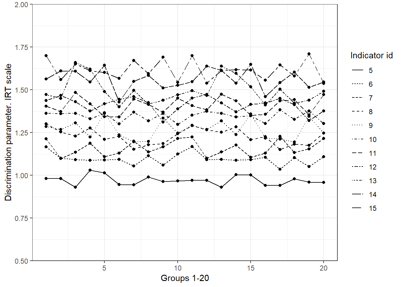
Figure 5.1: Discrimination parameters that seem to fulfil MI. Simulated data. We see very little fluctuation from one group to another
ggplot(irt_MIa_nonmi,aes(x=data,y=value,group=var_id)) + geom_point()  +
  geom_line(aes(linetype=as.factor(var_id))) +
  xlab("Groups 1-20") + ylab("Discrimination parameter. IRT scale") +
  labs(linetype='Indicator id') +
  scale_y_continuous( limits = c(.5,2), expand = c(0,0), breaks = seq(.5, 2, .25) ) +
theme_bw() 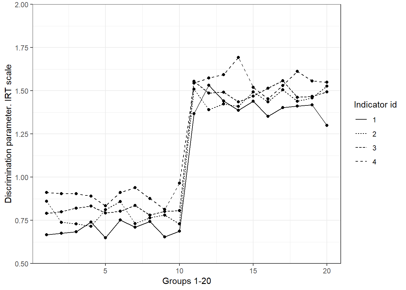
Figure 5.2: Discrimination parameters that do not seem to fulfil MI. Simulated data. We see a lot of fluctuation from groups 11-20 relative to 1-10
Figures 5.3 and 5.4 plot the values of the severity parameter for the items that are likely to be invariant across all groups and for the items that seem to violate MI, respectively. The severity parameters range between 0 and 3 standard deviations. As discussed in Chapter 4, this is the expected behaviour when looking at low standard of living. The items in plot 5.3 are very stable across groups. In contrast the severity parameters change a lot for groups 11 to 20 in comparison with the first ten groups (Figure 5.4). It seems, therefore, that these items are non-invariant, at least, between these two clusters. The severity parameter is tied with the intercept of a factor model (See Chapter 4). It indicates the mean value of deprivation for each item given the latent value of poverty. Different means are a violation of strong MI, and therefore is undesirable. In poverty research indicates the case where an indicator is a more/less severe manifestation of poverty when comparing two or more groups. In other words, it is an indication of when an indicator of a given society might be too severe to measure poverty in another. This is explained further using the real data example.
ggplot(irt_MIb_mi,aes(x=data,y=value,group=var_id)) + geom_point()  +
  geom_line(aes(linetype=as.factor(var_id))) +
  xlab("Groups 1-20") + ylab("Severity parameter. IRT scale") +
  labs(linetype='Indicator id') +
  scale_y_continuous( limits = c(0,4), expand = c(0,0), breaks = seq(0, 4, .5) ) +
theme_bw() 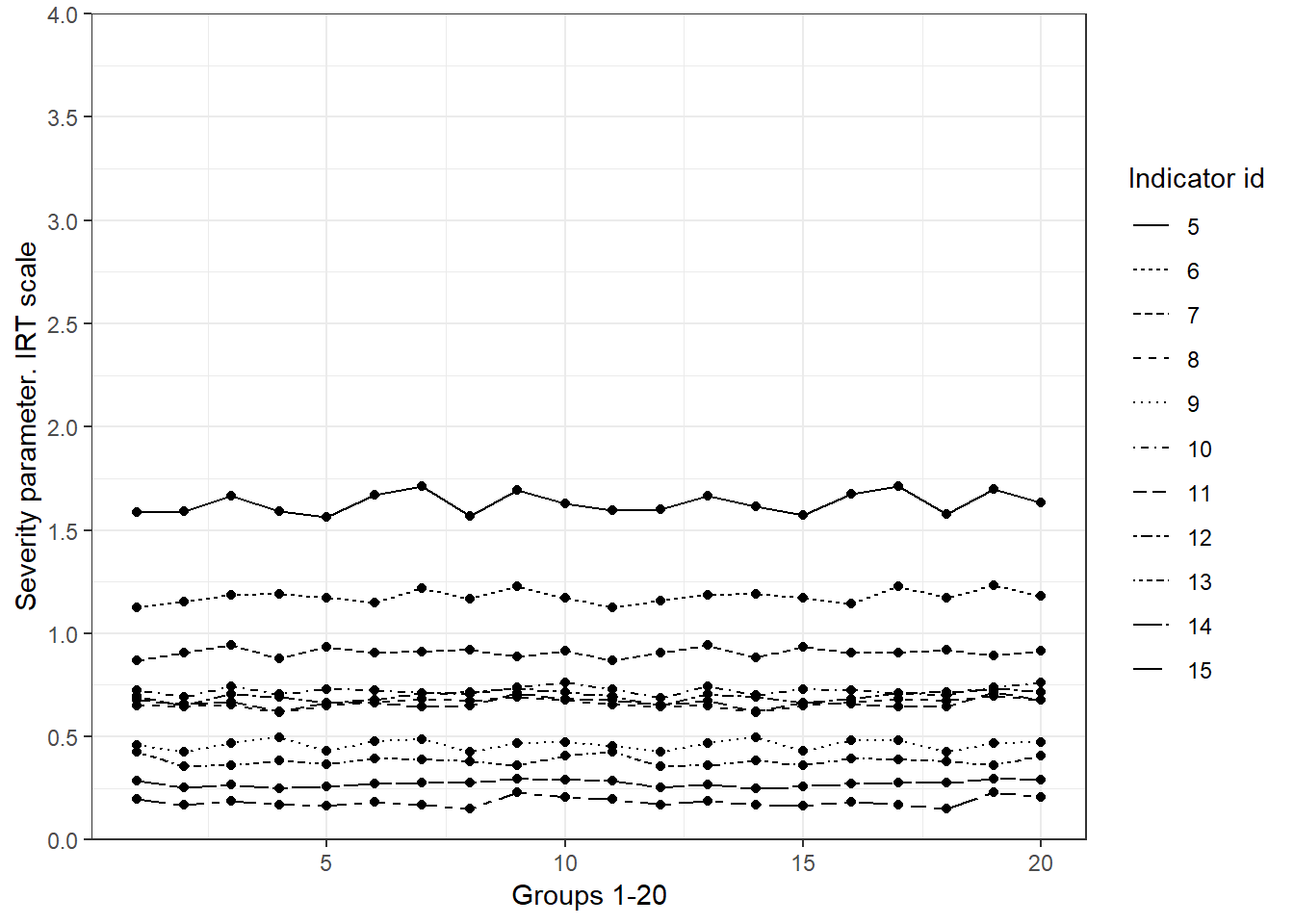
Figure 5.3: Severity parameters that seem to fulfil MI. Simulated data. We see very little fluctuation from one group to another
ggplot(irt_MIb_nonmi,aes(x=data,y=value,group=var_id)) + geom_point()  +
  geom_line(aes(linetype=as.factor(var_id))) +
  xlab("Groups 1-20") + ylab("Severity parameter. IRT scale") +
  labs(linetype='Indicator id') +
  scale_y_continuous( limits = c(0,4), expand = c(0,0), breaks = seq(1, 4, .5) ) +
theme_bw() 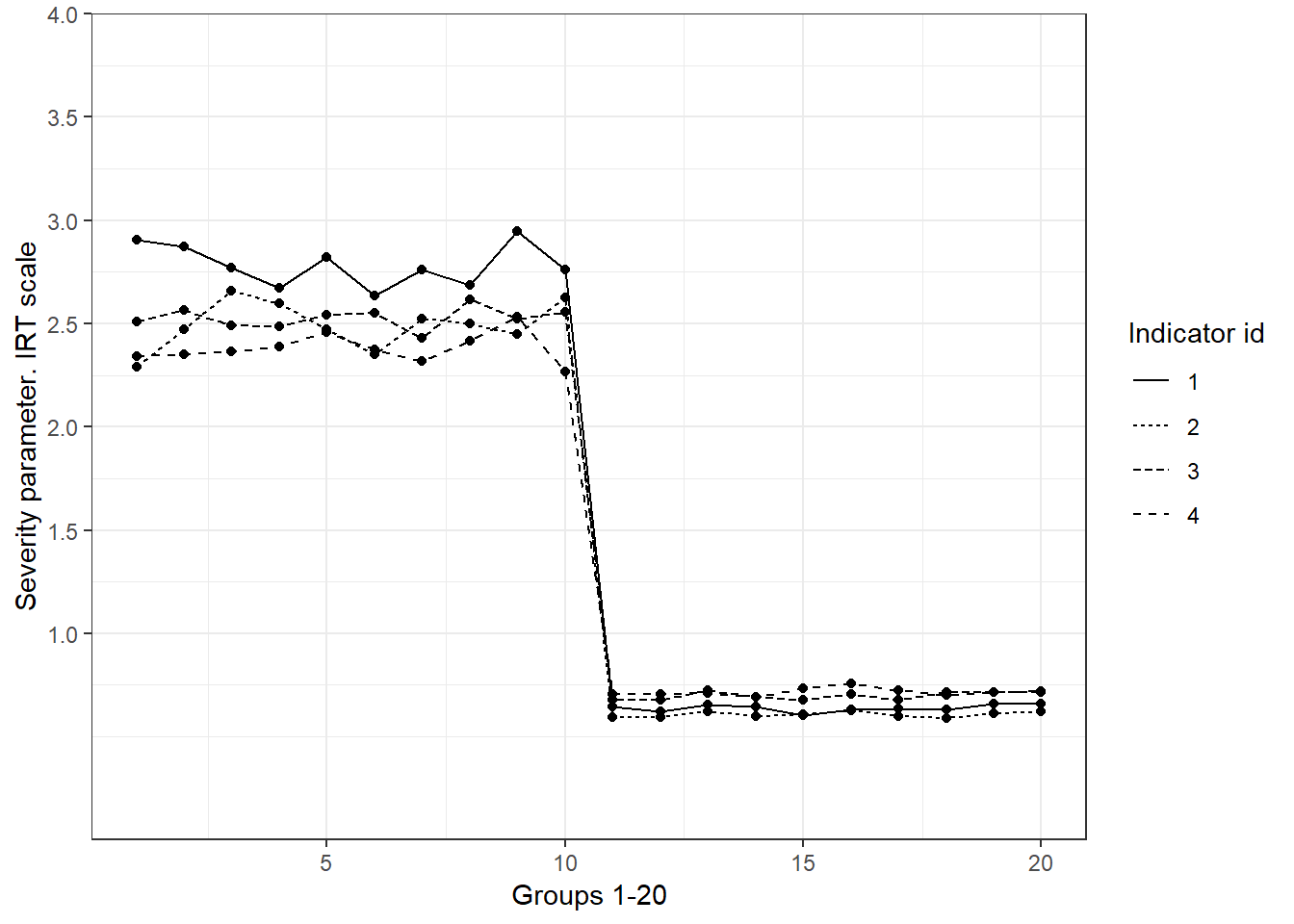
Figure 5.4: Severity parameters that do not seem to fulfil MI. Simulated data. We see a lot of fluctuation from groups 11-20 relative to 1-10
5.3 Methods for the assessment of Measurement Invariance
Measurement Invariance is formally examined by comparing the extent two which the parameters of a measurement model are similar between two or more groups/periods. The measurement model can be a unidimensional or a multidimensional factor model. That is, it can be seen as a formal assessment of the visual inspection shown in the previous section. The literature proposes two main methods to analyse MI: Multiple Group Factor Analysis (MGFA) and the Alignment Method (AM). The rationale behind both methods is the same, start from a measurement model with some free parameters (configural model, for example) and then move toward a model with fixed parameters (strong MI where loadings and thresholds are fixed across groups). The different models are contrasted using both absolute statistics of fit such as Chi-Square and relative statistics of fit like RMSEA and TLI, CFI. Based on these statistics researchers conclude whether the same model holds for two different groups.
ud_1<-read.table("UD_data_2_1.dat")
ud_1$data<-2
ud_2<-read.table("UD_data_1_1.dat")
ud_2$data<-1
ud_1and2<-rbind(ud_1,ud_2)
head(ud_1and2)
## V1 V2 V3 V4 V5 V6 V7 V8 V9 V10 V11 V12 V13 V14 V15 V16 data
## 1 0 1 0 1 1 0 0 1 0 0 0 0 1 1 1 2 2
## 2 0 0 0 0 0 0 0 0 0 0 0 0 0 0 0 2 2
## 3 1 1 1 1 1 1 0 0 1 1 1 0 1 1 1 2 2
## 4 0 0 0 0 0 0 0 0 0 0 0 0 0 0 0 1 2
## 5 0 0 0 0 0 0 0 0 0 0 0 0 0 0 0 1 2
## 6 0 0 0 1 0 0 0 0 0 0 0 0 0 1 1 2 2write.table(ud_1and2, file="ud_1and2.dat", col.names = F)5.3.1 Multiple Group Factor Analysis
Multiple Group Factor Analysis had been the classic method to assess MI. To illustrate how it works on Mplus (“MI_analysis_du_configural1and2.inp”), data for group 1 and group 11 (“ud_1and2.dat”) will be used to go through the different steps involved in testing MI. The first step consist in testing the hypothesis that a configural model holds between these two groups, i.e. whether the same unidimensional model holds leaving the loadings and thresholds free across groups. The syntax is displayed below. The syntax is very similar to the one used to fit a unidimensional Confirmatory Factor Model (CFA) following a two-parameter IRT model. One needs to tell Mplus the groups in question (GROUPING) and save the results of the Chi-square test to contrast out model with the models with fixed loadings and thresholds. It is also very important to request the Modification Indices, which tell which parameters are the sources of model miss fit and therefore the cause of violating more strict forms of MI. In this example, the mean of the latent variable is fixed to one given that those value were used to simulate these data.
test <- mplusObject(
TITLE = "Multiple Group Analysis;",
VARIABLE = "
Name = id V1-V16 data;
Missing are all (-9999) ;
usevariables = V1-V15;
categorical = V1-V15;
GROUPING = data (1=ONE 2=TWO);",

ANALYSIS="ESTIMATOR IS WLSMV;
PARAMETERIZATION=THETA;",

SAVEDATA= "DIFFTEST=Configural.dat;",

OUTPUT = "STDYX MODINDICES (3.84);",

MODEL = "

! Factor loadings all estimated
F BY V1-V15* (L1-L15);

! Item thresholds all free
[v1$1-v15$1*] (T1-T15);

! Item residual variances all fixed=1
V1-V15@1;

! Factor mean=0 and variance=1 for identification
[f@0]; f@1;

!!! CONFIGURAL MODEL FOR ALTERNATIVE GROUP
MODEL TWO:  ! Factor loadings all estimated

F BY V1-V15*;

! Item thresholds all free
[v1$1-v15$1*];

! Item residual variances all fixed=1
V1-V15@1;

! Factor mean=0 and variance=1 for identification
[f@0]; f@1;")

res <- mplusModeler(test, modelout = "MI_analysis_du_configural1and2.inp",
                    writeData = "never",
                    hashfilename = FALSE,
                    dataout="ud_1and2.dat", run = 1L)
##
## Running model: MI_analysis_du_configural1and2.inp
## System command: C:\WINDOWS\system32\cmd.exe /c cd "." && "Mplus" "MI_analysis_du_configural1and2.inp"
## Reading model: MI_analysis_du_configural1and2.outThe fit of the model (“MI_analysis_du_configural1and2.inp”) is shown below. The fit of the model is very good. Under the Chi-Square test the model is not rejected and the relative statistics of fit point in the same direction. However, this only a reference that allow us to inspect metric (weak) MI. Should the configural model is rejected, then comparing both poverty indices very likely lead to incorrect conclusion about both prevalence and severity of poverty.
fitstats<-c(TLI=res$results$summaries$TLI,
            CFI=res$results$summaries$CFI,
            Chisq=res$results$summaries$ChiSqM_PValue,
            RMSEA=res$results$summaries$RMSEA_Estimate)
fitstats
## TLI CFI Chisq RMSEA
## 1.0000 1.0000 0.0133 0.0070The Mplus input of the metric MI model, free threshold but fixed loadings, is displayed below (“MI_metricanalysis_du_1and2.inp”). To compare the fit of the configural model against the metric model it is necessary to call for the information stored in “DIFFTEST=Configural.dat;”. The main difference between these INPUT INSTRUCTIONS and the configural model is that the loadings of the 15 items are fixed -equal across groups-. Therefore, the model will fit such assumption to the data and see whether it holds or not.
test <- mplusObject(
TITLE = "Multiple Group Analysis (Metric);",
VARIABLE = "
Name = id V1-V16 data;
Missing are all (-9999) ;
usevariables = V1-V15;
categorical = V1-V15;
GROUPING = data (1=ONE 2=TWO);",

ANALYSIS="ESTIMATOR IS WLSMV;
PARAMETERIZATION=THETA;
DIFFTEST= Configural.dat;",

SAVEDATA= "DIFFTEST=MetricA.dat;",

OUTPUT = "STDYX MODINDICES (3.84);",

MODEL = "

! Factor loadings all estimated
 F BY V1-V15* (L1-L15);

! Item thresholds all free
[v1$1-v15$1*] (T1-T15);

! Item residual variances all fixed=1
V1-V15@1;

! Factor mean=0 and variance=1 for identification
[f@0]; f@1;

!!! CONFIGURAL MODEL FOR ALTERNATIVE GROUP
MODEL TWO:  ! Factor loadings all estimated

 F BY V1-V15* (L1-L15);

! Item thresholds all free
[v1$1-v15$1*];

! Item residual variances all fixed=1
V1-V15@1;

! Factor mean=0 and variance=1 for identification
[f@0]; f*;")

res <- mplusModeler(test, modelout = "MI_metric_analysis_du_configural1and2.inp",
                    writeData = "never",
                    hashfilename = FALSE,
                    dataout="ud_1and2.dat", run = 1L)
##
## Running model: MI_metric_analysis_du_configural1and2.inp
## System command: C:\WINDOWS\system32\cmd.exe /c cd "." && "Mplus" "MI_metric_analysis_du_configural1and2.inp"
## Reading model: MI_metric_analysis_du_configural1and2.outThe Chi-Square Test for Difference Testing in the output of the metric MI analysis leads to the rejection of the model (\(Chi-Square<.05\)). There is also a drop in the value of the relative statistics of fit TLI and CFI. These two suggest that although the model is relatively adequate, there is a loss after fixing the loadings across groups. This is expected given that the loadings of groups 1 and 11 are very different for some of the items.
fitstats<-c(TLI=res$results$summaries$TLI,
            CFI=res$results$summaries$CFI,
            Chisq=res$results$summaries$ChiSqM_PValue,
            RMSEA=res$results$summaries$RMSEA_Estimate,
            ChisqDIFF=res$results$summaries$ChiSqDiffTest_PValue)
fitstats
## TLI CFI Chisq RMSEA ChisqDIFF
## 0.992 0.993 0.000 0.031 0.000The modification indices of the metric model provide information about the parameters that make the main contribution to the inadequate model fit. Figure 5.2 suggested that indicators 1-4 were very likely to be non-invariant. The modification indices confirm that indeed these items are the main sources of the discrepancy between the two groups. Without prior knowledge or a clear theory of why these four items have non-invariant loadings, the suggestion would be to let these four loadings free and re-assess metric invariance. Otherwise, the alternative would be dropping these four indicators and re-examine metric MI.
res\(results\)mod_indices[1:15,]
To assess whether partial metric MI holds, the loadings of the four items in question (1-4) were no longer fixed between groups. The syntax is omitted but the output (“mi_metricanalysis_b_du_1and2.out”) is shown below. The Chi-Square Test for Difference Testing suggest that partial metric invariance holds. Indicating that it is feasible to proceed and conduct the examination of Strong MI (scalar MI).
test <- mplusObject(
TITLE = "Multiple Group Analysis (MetricB);",
VARIABLE = "
Name = id V1-V16 data;
Missing are all (-9999) ;
usevariables = V1-V15;
categorical = V1-V15;
GROUPING = data (1=ONE 2=TWO);",

ANALYSIS="ESTIMATOR IS WLSMV;
PARAMETERIZATION=THETA;
DIFFTEST= Configural.dat;",

SAVEDATA= "DIFFTEST=MetricB.dat;",

OUTPUT = "STDYX MODINDICES (3.84);",

MODEL = "

! Factor loadings all estimated
 F BY V1-V15* (L1-L15);

! Item thresholds all free
[v1$1-v15$1*] (T1-T15);

! Item residual variances all fixed=1
V1-V15@1;

! Factor mean=0 and variance=1 for identification
[f@0]; f@1;

!!! CONFIGURAL MODEL FOR ALTERNATIVE GROUP
MODEL TWO:

 F BY V1-V15* (L1a L2a L3a L4a L5-L15);

! Item thresholds all free
[v1$1-v15$1*];

! Item residual variances all fixed=1
V1-V15@1;

! Factor mean=0 and variance=1 for identification
[f@0]; f*;")

res <- mplusModeler(test, modelout = "MI_metricanalysis_B_du_1and2.inp",
                    writeData = "never",
                    hashfilename = FALSE,
                    dataout="ud_1and2.dat", run = 1L)
##
## Running model: MI_metricanalysis_B_du_1and2.inp
## System command: C:\WINDOWS\system32\cmd.exe /c cd "." && "Mplus" "MI_metricanalysis_B_du_1and2.inp"
## Reading model: MI_metricanalysis_B_du_1and2.outfitstats<-c(TLI=res$results$summaries$TLI,
CFI=res$results$summaries$CFI,
Chisq=res$results$summaries$ChiSqM_PValue,
RMSEA=res$results$summaries$RMSEA_Estimate,
ChisqDIFF=res$results$summaries$ChiSqDiffTest_PValue)
fitstats## TLI CFI Chisq RMSEA ChisqDIFF
## 1.0000 1.0000 0.4639 0.0010 1.0000In order to assess scalar invariance it is necessary to hold all the thresholds (intercepts) equal across groups.
test <- mplusObject(
TITLE = "Multiple Group Analysis (Scalar);",
VARIABLE = "
Name = id V1-V16 data;
Missing are all (-9999) ;
usevariables = V1-V15;
categorical = V1-V15;
GROUPING = data (1=ONE 2=TWO);",
ANALYSIS="ESTIMATOR IS WLSMV;
PARAMETERIZATION=THETA;
DIFFTEST= MetricB.dat;",
SAVEDATA= "DIFFTEST=Scalar.dat;",
OUTPUT = "STDYX MODINDICES (3.84);",
MODEL = "
! Factor loadings all estimated
F BY V1-V15* (L1-L15);
! Item thresholds all free
[v1$1-v15$1*] (T1-T15);
! Item residual variances all fixed=1
V1-V15@1;
! Factor mean=0 and variance=1 for identification
[f@0]; f@1;
!!! CONFIGURAL MODEL FOR ALTERNATIVE GROUP
MODEL TWO:
F BY V1-V15* (L1a L2a L3a L4a L5-L15);
! Item thresholds all fixed
! Item residual variances all fixed=1
V1-V15@1;
! Factor mean=0 and variance=1 for identification
[f@0]; f*;")
res <- mplusModeler(test, modelout = "MI_scalaranalysis_du_1and2.inp",
writeData = "never",
hashfilename = FALSE,
dataout="ud_1and2.dat", run = 1L)##
## Running model: MI_scalaranalysis_du_1and2.inp
## System command: C:\WINDOWS\system32\cmd.exe /c cd "." && "Mplus" "MI_scalaranalysis_du_1and2.inp"
## Reading model: MI_scalaranalysis_du_1and2.outThe output below (“mi_scalaranalysis_du_1and2.out”) indicates that partial scalar invariance holds. It seems that for this data, it is just necessary to let the loadings of the first four items free to achieve partial scalar invariance. This suggests that after considering differences in slope the means between groups are equivalent. This does no necessarily mean that the scale is fully invariant, the effect of the first four items could lead to incorrect conclusions when comparing poverty levels between these two groups. Next section discusses the meaning of threshold non-invariance in the context of poverty research, as this topic connects with scale equating.
fitstats<-c(TLI=res$results$summaries$TLI,
            CFI=res$results$summaries$CFI,
            Chisq=res$results$summaries$ChiSqM_PValue,
            RMSEA=res$results$summaries$RMSEA_Estimate,
            ChisqDIFF=res$results$summaries$ChiSqDiffTest_PValue)
fitstats
## TLI CFI Chisq RMSEA ChisqDIFF
## 0.989 0.989 0.000 0.038 0.000After fixing the thresholds of the first four items partial scalar invariance holds (\(Chi-square>.05\)). This would mean that in order to meet exact scalar invariance the four items in question must be dropped from the index. This is, of course, not ideal as most of the time poverty indices have few items to choose from.
test <- mplusObject(
TITLE = "Multiple Group Analysis (ScalarB);",
VARIABLE = "
Name = id V1-V16 data;
Missing are all (-9999) ;
usevariables = V1-V15;
categorical = V1-V15;
GROUPING = data (1=ONE 2=TWO);",

ANALYSIS="ESTIMATOR IS WLSMV;
PARAMETERIZATION=THETA;
DIFFTEST= MetricB.dat;",

SAVEDATA= "DIFFTEST=ScalarB.dat;",

OUTPUT = "STDYX MODINDICES (3.84);",

MODEL = "

! Factor loadings all estimated
 F BY V1-V15* (L1-L15);

! Item thresholds all free
[v1$1-v15$1*] (T1-T15);

! Item residual variances all fixed=1
V1-V15@1;

! Factor mean=0 and variance=1 for identification
[f@0]; f@1;

!!! CONFIGURAL MODEL FOR WOMEN ALTERNATIVE GROUP
MODEL TWO:

F BY V1-V15* (L1a L2a L3a L4a L5-L15);

! Item thresholds four first fixed
[v1$1-v4$1*];

! Item residual variances all fixed=1
V1-V15@1;

! Factor mean=0 and variance=1 for identification
[f@0]; f*;")

res <- mplusModeler(test, modelout = "MI_scalaranalysis_B_du_1and2.inp",
                    writeData = "never",
                    hashfilename = FALSE,
                    dataout="ud_1and2.dat", run = 1L)
##
## Running model: MI_scalaranalysis_B_du_1and2.inp
## System command: C:\WINDOWS\system32\cmd.exe /c cd "." && "Mplus" "MI_scalaranalysis_B_du_1and2.inp"
## Reading model: MI_scalaranalysis_B_du_1and2.outfitstats<-c(TLI=res$results$summaries$TLI,
CFI=res$results$summaries$CFI,
Chisq=res$results$summaries$ChiSqM_PValue,
RMSEA=res$results$summaries$RMSEA_Estimate,
ChisqDIFF=res$results$summaries$ChiSqDiffTest_PValue)
fitstats## TLI CFI Chisq RMSEA ChisqDIFF
## 1.0000 1.0000 0.7059 0.0000 0.96115.3.2 The alignment method
Multiple Group Factor Analysis has some disadvantages in real-data settings. In a real-data situation, researchers will have to fit a number of models to have an idea of the different sources of non-invariance. This is time-consuming and compromises the reproducibility of the findings given that another researcher might use different criteria to go through the modification indices. Another problem is that the MGFA is not feasible for many groups. Another disadvantage, when using Chi-Square, is that the models will be almost always rejected with large samples and researchers, therefore, have to work with rules of thumb to assess sufficient changes in TLI or CFI.
The alignment method has been put forward to overcome some of the drawbacks of MGFA. In particular, it simplifies the assessment of MI when having many groups. This method is under constant development but it aims to estimate means and variances of the latent factor conditional on a minimum level of MI. That means that it does not requires exact MI and aims at approximately MI. The alignment method therefore seeks an optional degree of measurement invariance given the data. The alignment method starts from the assumption that the configural model will be better that the fully scalar model. Once a configural model is fitted (M0), then the alignment method looks for a model that is equally as good as M0 but with some fixed parameters. By minimizing the loss function due to non-invariant parameters, the alignment method estimates factor means that are comparable conditional on the approximately invariant model.
temp = list.files(pattern="UD_data_.*.dat")
myfiles = lapply(temp, read.table)
myfiles<-myfiles[-11]
myfiles<-myfiles[-21]
data<-do.call(rbind,myfiles)
data$data<-rep(1:20,each=5000)
write.table(data,file="UD_MI_AM.dat", col.names = F)
To introduce the key aspects of the alignment method, this section relies on the simulated data generated for the 20 groups. A data set was created containing the 15 indicators for each case in the sample (\(n=5000\)) for each group (“UD_MI_AM.dat”). The alignment method is easily implemented on Mplus using the INPUT INSTRUCTIONS below (“UD_MI_AM.inp”). Mplus requires the name of the variable containing the group ids as well as the total number of groups (classes). Then a unidimensional factor model is specified. Mplus produces some useful plots to visualise, in this case, the IRT parameters of the model. This is similar to Figures 5.1 to 5.4.
INPUT INSTRUCTIONS

  Data:
    File is UD_MI_AM.dat ;
  Variable:
    Names are id V1-V16 data;
    Missing are all (-9999) ;

  usevariables = V1-V15;

  categorical = V1-V15;

  classes = c(20);
  knownclass = c(data = 1 2 3 4 5 6 7 8 9 10
                         11 12 13 14 15 16 17 18 19 20);


  Analysis:  type = mixture;
            estimator = ml;
            alignment = free;
            ALGORITHM=INTEGRATION;
            Process=8;

  model:
            %overall%
            f by V1-V15;


    output:
            tech1 tech8 align;

    plot:
            type = plot2;
The results of the alignment method are displayed below. In rows the output indicates whether the parameter is variant or non-invariant (in brackets). The number corresponds to the number of the group. These findings suggest that all the thresholds are invariant and that all the loadings of items 5 to 15 (V5 to V20) are invariant. The loadings of the first four items are non-invariant. These results are consistent with the findings of the MGFA. However, in this case the analysis is performed for the 20 groups and only one model needed to be fitted to the data. The alignment method indicates that for these data is possible to minimize non-invariance if the loadings of items 1 to 4 (V1 to V4) are not fixed for groups 11 to 20. Therefore, the results suggest that partial scalar invariance holds for this simulated example.
The alignment method suggest that the 20 poverty indices are comparable once the non-invariance of the loadings of the first four items is accounted by for.
APPROXIMATE MEASUREMENT INVARIANCE (NONINVARIANCE) FOR GROUPS

 Intercepts/Thresholds
   V1$1        1 2 3 4 5 6 7 8 9 10 11 12 13 14 15 16 17 18 19 20
   V2$1        1 2 3 4 5 6 7 8 9 10 11 12 13 14 15 16 17 18 19 20
   V3$1        1 2 3 4 5 6 7 8 9 10 11 12 13 14 15 16 17 18 19 20
   V4$1        1 2 3 4 5 6 7 8 9 10 11 12 13 14 15 16 17 18 19 20
   V5$1        1 2 3 4 5 6 7 8 9 10 11 12 13 14 15 16 17 18 19 20
   V6$1        1 2 3 4 5 6 7 8 9 10 11 12 13 14 15 16 17 18 19 20
   V7$1        1 2 3 4 5 6 7 8 9 10 11 12 13 14 15 16 17 18 19 20
   V8$1        1 2 3 4 5 6 7 8 9 10 11 12 13 14 15 16 17 18 19 20
   V9$1        1 2 3 4 5 6 7 8 9 10 11 12 13 14 15 16 17 18 19 20
   V10$1       1 2 3 4 5 6 7 8 9 10 11 12 13 14 15 16 17 18 19 20
   V11$1       1 2 3 4 5 6 7 8 9 10 11 12 13 14 15 16 17 18 19 20
   V12$1       1 2 3 4 5 6 7 8 9 10 11 12 13 14 15 16 17 18 19 20
   V13$1       1 2 3 4 5 6 7 8 9 10 11 12 13 14 15 16 17 18 19 20
   V14$1       1 2 3 4 5 6 7 8 9 10 11 12 13 14 15 16 17 18 19 20
   V15$1       1 2 3 4 5 6 7 8 9 10 11 12 13 14 15 16 17 18 19 20

 Loadings for F
   V1          1 2 3 4 5 6 7 8 9 10 (11) (12) (13) (14) (15) (16) (17) (18) (19) (20)
   V2          1 2 3 4 5 6 7 8 9 10 (11) (12) (13) (14) (15) (16) (17) (18) (19) (20)
   V3          1 2 3 4 5 6 7 8 9 10 (11) (12) (13) (14) (15) (16) (17) (18) (19) (20)
   V4          1 2 3 4 5 6 7 8 9 10 (11) (12) (13) (14) (15) (16) (17) (18) (19) (20)
   V5          1 2 3 4 5 6 7 8 9 10 11 12 13 14 15 16 17 18 19 20
   V6          1 2 3 4 5 6 7 8 9 10 11 12 13 14 15 16 17 18 19 20
   V7          1 2 3 4 5 6 7 8 9 10 11 12 13 14 15 16 17 18 19 20
   V8          1 2 3 4 5 6 7 8 9 10 11 12 13 14 15 16 17 18 19 20
   V9          1 2 3 4 5 6 7 8 9 10 11 12 13 14 15 16 17 18 19 20
   V10         1 2 3 4 5 6 7 8 9 10 11 12 13 14 15 16 17 18 19 20
   V11         1 2 3 4 5 6 7 8 9 10 11 12 13 14 15 16 17 18 19 20
   V12         1 2 3 4 5 6 7 8 9 10 11 12 13 14 15 16 17 18 19 20
   V13         1 2 3 4 5 6 7 8 9 10 11 12 13 14 15 16 17 18 19 20
   V14         1 2 3 4 5 6 7 8 9 10 11 12 13 14 15 16 17 18 19 20
   V15         1 2 3 4 5 6 7 8 9 10 11 12 13 14 15 16 17 18 19 20
5.4 Real-data analysis of Measurement Invariance
Strong (or Scalar) measurement invariance is unlikely to hold when working with real data. The analysis of MI is fairly new in poverty research that there is no agreement about what the desirable level of MI should be.@Guio2017 found partial scalar MI using the EU-SILC data and Najera (2016) found partial scalar MI for the official Mexican multidimensional measure. Both exercises conclude that the ideal is scalar MI but that in practice partial scalar is a more sensible standard. Both non-invariant thresholds and loadings are likely to appear in real-data analyses but given that differences in difficulty -thresholds- could be more explicitly accounted by for in scale equating -next chapter- one sensible recommendation is to maximize metric invariance and then move onto partial scalar invariance.
The INPUT INSTRUCTIONS of the MI analysis of the FRS data (“FRS_mplusprep.dat”) are shown below. The data set contains all the 25 deprivation indicators, sampling weights (gross4) and the household id (id). There is data available for ten periods (2004/2005 to 2013/2104). However, four variables were replaced by another four in 2011. Therefore, the MI analysis is performed using the 17 common variables across both periods -next chapter concerns with the issue of equating and scaling measures with different and non-invariant indicators). The classes in the INPUT INSTRUCTIONS are the 10 years (ordered were 1=2004/2005, …, 10=2013-2014). For the purposes of the illustration cluster sampling is assumed but we recommend checking the Mplus manual for deeper understanding of working with complex samples.
INPUT INSTRUCTIONS

  Data:
    File is FRS_mplusprep.dat ;
  Variable:
    Names are
       gross4 FRSYear dep_ADDDEC dep_ADDEPLES dep_ADDHOL
       dep_ADDINS dep_ADDMEL dep_ADDMON dep_ADDSHOE dep_ADEPFUR
       dep_AF1 dep_AFDEP2 dep_HOUSHE1 dep_CDELPLY dep_CDEPBED
       dep_CDEPCEL dep_CDEPEQP dep_CDEPHOL dep_CDEPLES
       dep_CDEPSUM dep_CDEPTEA dep_CDEPTRP dep_CPLAY
       dep_CDEPACT dep_CDEPVEG dep_CDPCOAT dep_ADBTBL id;
    Missing are all (-9999) ;

  usevariables = dep_ADDDEC  dep_ADDHOL dep_ADDINS
        dep_ADDMON  dep_ADEPFUR dep_AF1 dep_AFDEP2 dep_HOUSHE1
       dep_CDELPLY dep_CDEPBED dep_CDEPCEL dep_CDEPEQP dep_CDEPHOL
       dep_CDEPLES dep_CDEPTEA dep_CDEPTRP dep_CPLAY;

  categorical = dep_ADDDEC  dep_ADDHOL dep_ADDINS
        dep_ADDMON  dep_ADEPFUR dep_AF1 dep_AFDEP2 dep_HOUSHE1
       dep_CDELPLY dep_CDEPBED dep_CDEPCEL dep_CDEPEQP dep_CDEPHOL
       dep_CDEPLES dep_CDEPTEA dep_CDEPTRP dep_CPLAY;

  classes = c(10);
  knownclass = c(FRSYear = 1 2 3 4 5 6 7 8 9 10);

  weight=gross4;

  cluster=id;

  Analysis:  type = mixture complex;
            estimator = ml;
            alignment = fixed;
            ALGORITHM=INTEGRATION;
            Process=8;

  model:

            f by dep_ADDDEC  dep_ADDHOL dep_ADDINS
        dep_ADDMON  dep_ADEPFUR dep_AF1 dep_AFDEP2 dep_HOUSHE1
       dep_CDELPLY dep_CDEPBED dep_CDEPCEL dep_CDEPEQP
       dep_CDEPHOL dep_CDEPLES
       dep_CDEPTEA dep_CDEPTRP dep_CPLAY;


    output:
            tech1 tech8 align;

    plot:
            type = plot2;
One of the key outputs of the alignment method is displayed below and it shows which parameters are non-invariant (within brackets) for each year. For example, the intercept of DEP_ADDD non-invariant for group 1 and the intercepts of DEP_ADDH and DEP_ADDI are invariant. The results suggest that partial scalar MI holds. This can be achieved by using a subset of items with both invariant intercepts and loadings: DEP_ADDI, DEP_ADEP, DEP_AF1, DEP_AFDE, DEP_CDEPEQP, DEP_CDEPHOL, DEP_CDEPTRP and DEP_CPLA. There are other items that are almost fully invariant as they only violate MI in one group. At this point is worth noting that the alignment method finds the parameters that maximize approximate MI and, therefore, MGFA could be used to find more items that fulfill MI once other parameters have been fixed, this the advantage but also the disadvantage of the MGFA in that it allows the researcher to find that partial scalar MI models -if exists- that suits better the purposes of her research.
APPROXIMATE MEASUREMENT INVARIANCE (NONINVARIANCE) FOR GROUPS

 Intercepts/Thresholds
   DEP_ADDD$1  (1) 2 3 4 5 6 7 8 9 10
   DEP_ADDH$1  1 2 3 4 5 6 7 8 9 10
   DEP_ADDI$1  1 2 3 4 5 6 7 8 9 10
   DEP_ADDM$1  (1) (2) (3) (4) 5 6 7 8 9 (10)
   DEP_ADEP$1  1 2 3 4 5 6 7 8 9 10
   DEP_AF1$1   1 2 3 4 5 6 7 8 9 10
   DEP_AFDE$1  1 2 3 4 5 6 7 8 9 10
   DEP_HOUS$1  (1) (2) 3 4 5 6 7 8 9 10
   DEP_CDEL$1  (1) (2) (3) (4) (5) 6 7 8 9 10
   DEP_CDEP$1  1 2 3 4 5 6 7 8 9 10
   DEP_CDEP$1  1 2 3 4 5 6 7 8 9 10
   DEP_CDEP$1  1 2 3 4 5 6 7 8 (9) 10
   DEP_CDEP$1  (1) 2 3 4 5 6 7 8 9 10
   DEP_CDEP$1  1 2 3 4 5 6 7 8 9 (10)
   DEP_CDEP$1  1 2 3 4 5 6 7 8 9 10
   DEP_CDEP$1  1 2 3 4 5 6 7 8 9 10
   DEP_CPLA$1  1 2 3 4 5 6 7 8 9 10

 Loadings for F
   DEP_ADDD    (1) 2 3 4 5 6 7 8 9 10
   DEP_ADDH    (1) (2) (3) (4) 5 6 7 8 9 10
   DEP_ADDI    1 2 3 4 5 6 7 8 9 10
   DEP_ADDM    1 2 3 4 5 (6) 7 8 9 (10)
   DEP_ADEP    1 2 3 4 5 6 7 8 9 10
   DEP_AF1     1 2 3 4 5 6 7 8 9 10
   DEP_AFDE    1 2 3 4 5 6 7 8 9 10
   DEP_HOUS    1 2 (3) (4) 5 6 7 8 9 10
   DEP_CDEL    1 2 3 4 5 6 7 8 9 10
   DEP_CDEP    1 2 3 4 5 6 7 8 9 10
   DEP_CDEP    1 2 3 4 5 6 7 8 9 10
   DEP_CDEP    1 2 3 4 5 6 7 8 (9) 10
   DEP_CDEP    1 2 3 4 5 6 7 8 9 10
   DEP_CDEP    (1) 2 3 4 5 6 7 8 9 10
   DEP_CDEP    1 2 3 4 5 6 7 (8) (9) 10
   DEP_CDEP    1 2 3 4 5 6 7 8 9 10
   DEP_CPLA    1 2 3 4 5 6 7 8 9 10
One of the key purposes of the alignment method is to compare groups on the factor mean once approximate MI is met. The results suggest that the severity of child deprivation has remained pretty much the same. Years, 5 (2008/09), 6 (2009/10) and 7 (2010/11), however, have significantly smaller means compared with 2004/2005. This suggest that in the observed period and with these 17 indicators, child deprivation was at its lowest level in 2008/09 (pre-economic crisis). It seems that after the year 2010/11 severity increased and reached similar levels of the early 2000s.
FACTOR MEAN COMPARISON AT THE 5% SIGNIFICANCE LEVEL IN DESCENDING ORDER

 Results for Factor F

           Latent    Group      Factor
 Ranking    Class    Value       Mean     Groups With Significantly
                                          Smaller Factor Mean
     1         1         1       0.000    6 7 5
     2         4         4      -0.005    5
     3         3         3      -0.011    5
     4         9         9      -0.014    5
     5        10        10      -0.029
     6         8         8      -0.034
     7         2         2      -0.036
     8         6         6      -0.042
     9         7         7      -0.048
10 5 5 -0.065library(haven)
library(plyr)
D<-read_dta("FRS_mplusprep.dta")
if(D$FRSYear<=7) {
D$ds_uw<-rowSums(D[,c(3:23)],na.rm=TRUE)
} else {
rowSums(D[,c(3,5,6,8,10,11:19,21:27)],na.rm=TRUE)
}
ds_frs<-ddply(D,.(FRSYear), summarise, mean_ds=mean(ds_uw))
ds_frs$year<-c("2004/2005","2005/2006","2006/2007","2007/2008","2008/2009","2009/2010","2010/2011","2011/2012",
"2012/2013","2013/2014")
frs_raw<-data.frame(ds_raw=c(0.000 , -0.005, -0.011, -0.014, -0.029, -0.034, -0.036, -0.042, -0.048, -0.065), FRSYear=c(1,4,3,9,10,8,2,6,7,5))
ds_frs<-merge(ds_frs,frs_raw,by="FRSYear")Figure 5.5 plots the raw child deprivation score (0-17 count) and the adjusted factor score. When a scale is highly reliable and fully invariant, the raw mean and the factor score must be highly (negatively) correlated. The plot does not shows a clear correlation. The MI analysis suggested that several parameters need to be taken into account for the scale to be comparable over time. Whereas the raw deprivation score suggest that severity of deprivation has decreased over time (particularly after 2011), the MI analysis suggest that this is not the case as the scale lost comparability. Therefore, researchers relying on raw scores or any other transformation that does not takes into account non-invariance are likely to arrive to incorrect conclusions about the trends in child deprivation.
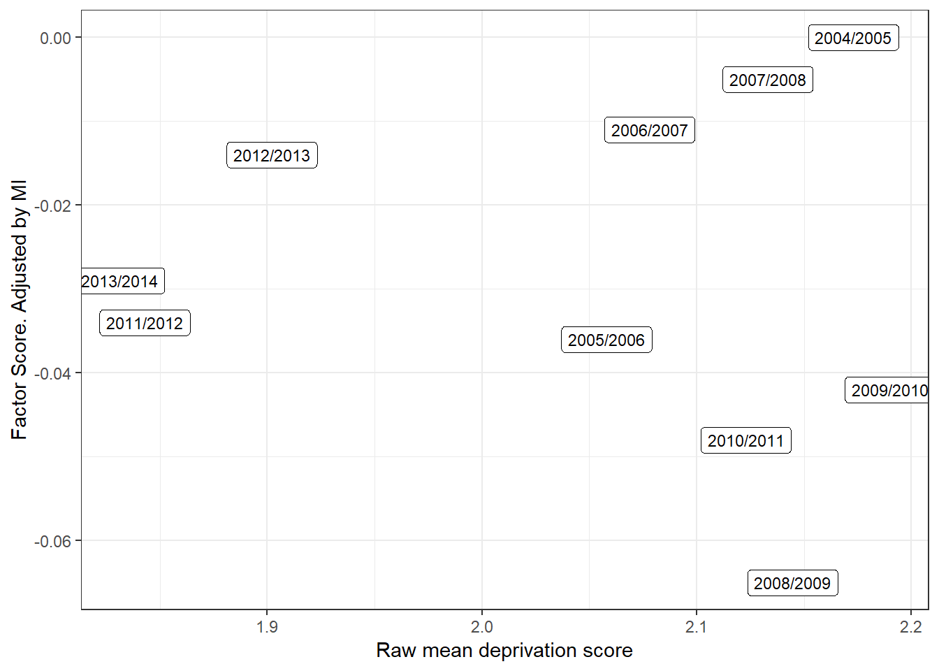
Figure 5.5: Scatter plot with a comparison of the raw mean child deprivation score (simple count) and the factor adjusted score. FRS data 2004-2013. The plot shows that there a great deal of discrepancy between the adjusted and the unadjusted severity scores. Conclusions about the depth of poverty are affected by the comparability of the data over time.
Prevalence weighting has been a means to consider the severity of item-level deprivation in the estimation of overall deprivation and poverty (???). This procedure consists in assigning more weight to those items that most people have in the society in question. As discussed in the chapter on Reliability, an index is self-weighting for high reliability values. Therefore, very little is gained when using differential weighting. However, when comparing groups or years weighting could help to improve the comparability of a measure as this procedure is directly associated with the difficulty/severity parameter. Adjusting by differences in severity is one way to improve comparisons across groups. The next chapter, therefore, focuses on how equating, linking and scaling can be used to make scales comparable.