Chapter 6 Scale equating and linking
Abstract
This chapter focuses on a framework to make scales comparable across groups, countries and time points. It describes the theory of scale equating which proposes that two or more indices, with some indicators in common but not necessarily the same, can be made comparable via modelling. The chapter focuses in one form of equating: Item Response Theory equating because it is widely used, and it fits more naturally with the whole rationale of the book. Several examples are used to illustrate the main concepts and its implementation in R.
6.1 Intuition to scale equating
Previous chapter introduces the sources affecting the comparability of different poverty indices and presents the concept and empirical implementation of measurement invariance. In poverty research, households are ranked according to some indicators of (low) material and social deprivation using survey or census data. The indicators in question have a structure (unidimensional or multidimensional, See chapter 1) for the general population. One problem is that such a measurement model might not be adequate for a different population (such as countries) or for a different year. We saw in previous chapter that in statistical terms this means that the measurement model is not equivalent across groups. We now know that, once a MI assessment has been conducted, poverty can be compared on the factor using the alignment method. This, however, might not be fully satisfactory for policy makers as the values of a standardized latent variable make little practical sense. Furthermore, it is unclear how to use these values to set a poverty line.
Another critical problem is that MI is adequate when scales have the same items and it does not solve the problem of working with scales that have different items or that have been upgraded in accordance with the living standards. Ideally, once measurement invariance is assessed researches would like to put everything into a meaningful metric and being able to compare measures that might have suffered from changes in its contents. Moreover, one question in poverty research is about how the severity of poverty is affected by changes in living standards and how this can be tractable using the available data. Thus, poverty measures need to be equated or equivalised in some way so that we can make meaningful comparisons across groups or time.
Scale or test equating is the answer from measurement theory to the problem of working with scales that are not necessarily equivalent across countries, time points, etc. The academic concern with making scores comparable has a history of more than 90 years (Holland, 2007). The modern development of the theory of scale equating can be traced back to the 1980s (Haebara, 1980; Kolen, 1988; Petersen, Cook, & Stocking, 1983). However, after the publication of Kolen & Brennan (2004)’s seminal book, this framework has become more accessible through software development and implemented in several fields and has been under constant development (Davier, 2010; González & Wiberg, 2017).
Educational testing has been the field at the forefront of scale equating. Admissions to universities often depend on the score of a test. But what if this test favours some students? and What if different versions of the tests are implemented? This poses a challenge for the admissions’ office for two students might have different scores but just because the tests had different difficulties, i.e. one was easier than other.
How does this problem translate to poverty measurement? There are two good examples to see this happening to our scales. According to Townsend (1979) poverty is relative across time and space. The space to identify the dimensions and indicators of poverty in the early 20th Century would look very different from the space of things and activities necessary to live with dignity in the 21st Century. For example, overcrowding and access to electricity were very good indicators of poverty in London but these days is no longer the case. That means that the two measure will have different deprivation indicators. So, what does it mean that someone in the early 20th century had a deprivation score equal to 6 relative to someone that has a score equal to 3 today? Is it possible to compare how severely deprived they are? And how this might or might not impact the prevalence rate?
This is a very crude example, but it helps to illustrate some of the challenges when comparing poverty overtime. However, in poverty research one common belief is that using the same indicators is sufficient to make valid comparisons across groups. Leaving aside the data collection and sampling issues associated with MI, we could think carefully about this assumption. Imagine that we use indicators of the early 20th to measure poverty today. Then we have two people with the same deprivation pattern- they lack electricity, cook with charcoal, and live in an overcrowded house. Hence, they have the same deprivation scores. In the early 20th century it would not be very difficult to find such conditions in a small random sample. However, these days this situation would denote acute material deprivation. But these two people will have the same deprivation score, so without equating they would be equally deprived. How sensible is this conclusion? Well, not very.
Scale equating aims at adjusting the differences in severity between tests and groups. The process of equating, given the response patterns, will notice that it is more difficult (as in Item Response Theory modelling) today being deprived of the items in question than 100 years ago. So, based on difficulty, the contemporary scale will be adjusted in terms of the early 20th Century’s scale. If the equating process is successful, it should make sense and a score equal 3 today would mean something more severe in terms of a score equal 3 100 years ago, i.e. it will be higher. The inflation of today’s score will be the result of equating and it will tell us a lot of useful information to adjust our conclusions about poverty and severity of deprivation.
The second example focuses on the practical use of equating. Statistical offices tend to update their indices overtime, or we tend to have countries with two different measures but with some common indicators. So, they drop so indicators and include some new indicators. This just adds to the frustration of policymakers and academics because comparability is lost. One way to tackle this problem is scale equating. Figure @(fig:changeEQ) displays a common situation in which the indicators have changed from measure A (Poverty) to measure B (Poverty B). There are seven items that appear in both measures and two items that were dropped and other two that were included.
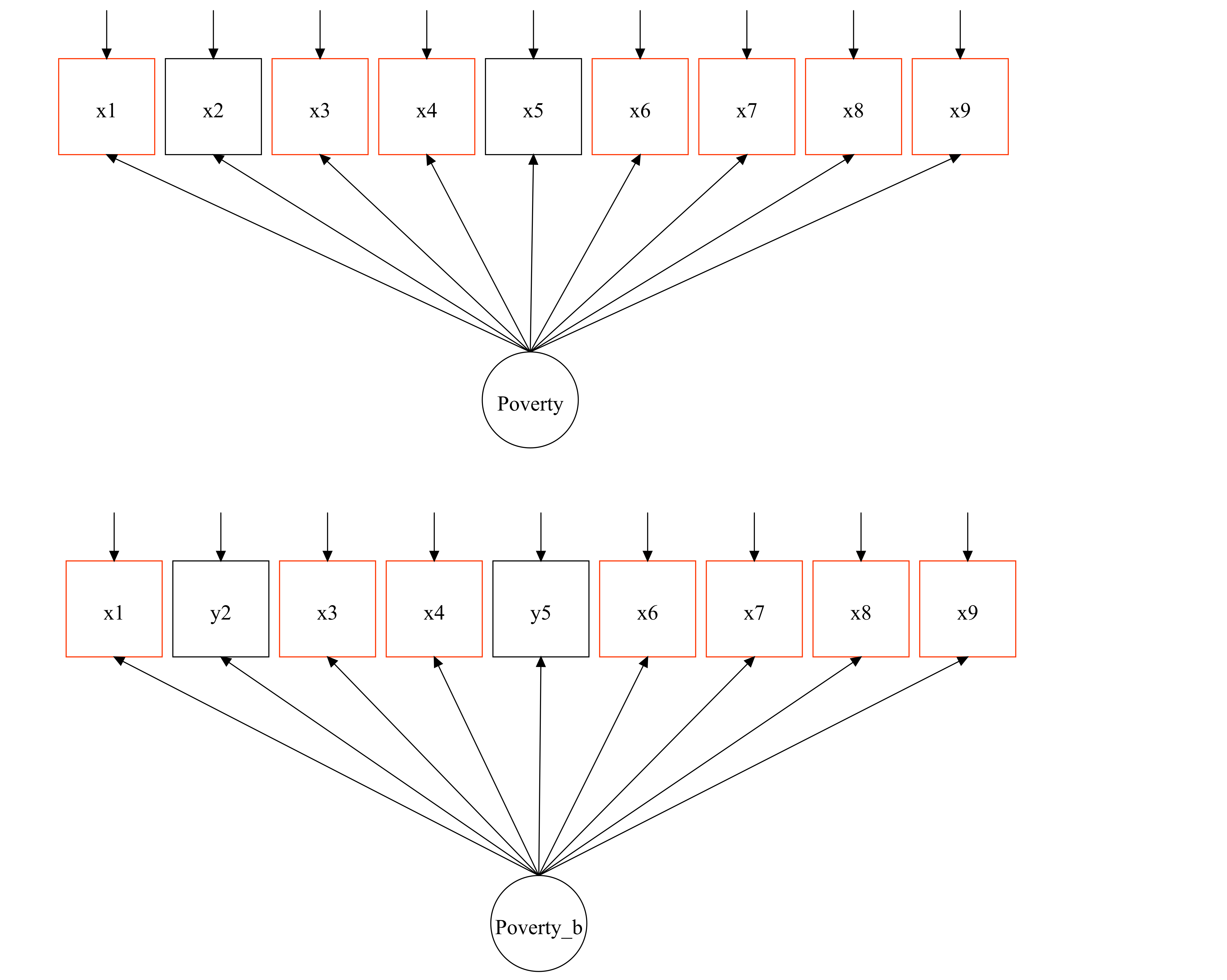
Figure 6.1: This figure shows the case in which there is a modification in the contents of a measure. In red there are the common items between the two measures
One crucial aspect of the example above is that if we have to tests with a common subset of items, then we can assess not only the effect of the updating of the scale but also, we could link both measures and make them comparable across time points. We will see that for scale equating to work we need to identify as many anchors as we can, i.e. items that respect measurement invariance across tests. In this case we have seven potential candidates. In the following we introduce formally the concepts and methods to conduct scale equating. We will, of course, discuss some limitations of this approach as it might be sensible in all situations or desirable.
6.2 Theory of scale equating [#Theoryequating]
6.2.1 Workflow in scale equating
Drawing upon Davier (2010), before formally introducing scale equating, we will present some of the stages involved in this process.
Two or more poverty indices (test forms using the vocabulary in scale equating): We will have two indices and one research question: How to measure and compare the latent poverty levels of the population regardless of which index we use.
Detecting confounding differences: The task is to measure the latent poverty levels by avoiding the confounding effect of using indices that look at more or less acute deprivation indicators with the effect of latent poverty. This implies figuring out the differences between the estimated severities/difficulties of the indicators and the underlying latent level of poverty.
Modelling the data generating process: Looking at different modelling alternatives, check their assumptions and assess how sensible using a given model is. There are several methods, observed score equating, IRT equating, kernel equating, etc.
Error in equating: All models are wrong and thus it is vital to assess the extent to which the results of our model are useless or reasonable given the errors of the parameters that are being estimated.
6.2.2 Theory of IRT scale equating
In this edition of this book, we will focus on one of the most widely used form of equating: Item Response Theory (IRT) equating because it is a framework that has been used for reliability analysis and fits more naturally with the kind of thinking behind this book: Poverty is a concept and its measurement is based on reflective models where deprivation is a cause of poverty. Thus, people have a latent level of poverty that produces observed deprivation scores.
Chapter 2 underline the importance of explicitly working with models and blueprints in multidimensional poverty measurement. We proposed in equation (2.1) a very simple model that looks as follows:
\[\begin{equation} \tag{2.1} \mathscr F = \{\mathscr X, F_{\theta} : \theta \in \Theta\} \end{equation}\]
where the variables \(x_1,...,x_n\) follow a certain distribution \(F_{\theta}\), which is indexed by a parameter \(\theta\) defined in the parameter space \(\Theta\). \(\mathscr F\) is a family of all probability distributions on \(\mathscr X\), which is just the set of all possible observed data.
We will borrow the formulation of González & Wiberg (2017) notation to formulate the equating model based on Item Response Theory, as this will be the method that we will use in the book, as it is consistent with the methods and rationale that we have used so far in the book.
For example, Item Response Theory (IRT) models, which are widely used in test equating, take the following general form:
\[\begin{equation} \tag{6.1} \mathscr F = {{0,1}, Bernoulli[\pi(\alpha_i, \omega_j)]:(\alpha_i, \omega_j) \in \mathbb{R} x \mathbb{R}} \end{equation}\]
For a two-parameter IRT model we would have \(x_{ij}\) denoting a binary deprivation indicator of an individual \(i\) who poverty is measured based on the index \(j\). That means that the probability of being deprived is given by: \((x_{ij} | \theta_i, a_j, b_j) \sim Bernoulli\), where \(\theta_i\) is person’s latent poverty, \(a_j\) is the discrimination of the item, \(b_j\) is the severity of the item. () is the item characteristic curve (ICC).
The key parameters in this example are thus \(\theta_i, a_j, b_j\). In the case that we have two indices \((j=2)\) we would like to link in some way the parameters of the first index (\(X\)) with the second index (\(Y\)). This could be achieved by estimating an IRT model for each index, extracting the parameters in question and then apply a linear equation to convert the IRT scores as:
\[\begin{equation} \tag{6.2} \theta_{yi} = A\theta_{xi} + B \end{equation}\]
To relate the parameters between the two tests we use the following:
\[\begin{equation} \tag{6.3} a_{yj} = a_{xj} / A \end{equation}\]
\[\begin{equation} \tag{6.3} b_{yj} = Ab_{xj} + B \end{equation}\]
where A and B are the equating coefficients and these need to be estimated using different methods such as mean-sigma, mean-geometric, Haebara, Stocking-Lord [González & Wiberg (2017); Davier2010]. Once these parameters have been estimated, the next step consists in putting the index \(X\) in terms of the index \(Y\). This process assumes that scores are equated considering the latent level of poverty which relates to observed score. There are two perspectives to do so: Observed-score equating and True-score equating (Kolen & Brennan, 2004). We explain these two very briefly:
Observed-score equating is based on the actual marginal score distributions (i.e. imagine a histogram of a deprivation score. This kind of equating uses the IRT model to adjust the score distributions across parallel forms, i.e. indices. To do so an observed score is calculated at each specified value of latent poverty level (remember that the metric of this variable is \(\theta \sim (0,\sigma^2)\)). This is summed/integrated across all levels of latent poverty to produce a marginal score distribution. The equipercentile is applied to establish the relationship between the two observed scores.
True-score equating draws on the idea of a true score from Classical Test Theory (CTT). The whole idea is that people with the same level of latent poverty \(\theta_j\) should have an equivalent true score, regardless the differences between tests. First, a latent poverty level (\(\theta_j\), where \(j=1\)) is associated with a true score via the Newton-Rapson method. Then the true score of the A index is mapped into the index B using the same latent poverty level (\(\theta_j\), where \(j=2\)). This procedure is often applied for each integer of the deprivation score.
6.3 Data and designs in test equating
One of the major challenges in equating is disentageling the differences in severity between tests from the differences in latent poverty levels across the populations subject to the measurement. Equating aims to correct differences in severity across test so we need a design that help us to assess the extent to which we are comparing populations with similar levels of latent poverty.
The simplest design is applying, for example, two different indices to the same population. So we can the latent values of poverty measured by each scale. However, this is not very useful because we often want to compare different populations or time points. One common solution to this problem is to use an anchor scale, i.e. the scores of the common items between populations. This will tell us the difference in latent poverty levels between two populations. It is essential that this anchor scales reflects the severity of the whole test. Below we briefly describe the different designs. We, however, note that only the last two designs are likely to make sanse in poverty research and we will focus on these two.
6.3.1 Single group design
This design uses a unique population. We could implement two scales A and B. If we measure each person in the sample using both forms we could easily equate the tests as we are measuring the same levels of latent poverty.
6.3.2 Equivalent groups design
Instead of applying the two measures to the population, equivalent groups design applies one scale to a random -representative- sample of the population and the second scale to a different sample.
6.3.3 Non Equivalent Groups with Anchor test Design
The simplest case of the Non Equivalent Groups with Anchor test Design (NEAT) consist in having two popualtions -sampled independently-. Poverty is measured using different scales (A and B) but there is a common anchor sub-index that is included in both A and B. In practice, we will have two countries with different indices but with a subset of common items. As we discussed in Section ??, it is not enough to use the same items but to make certain that the items respect measurement invariance. Another example of a NEAT design is when we have two measures in two different time points with common items in \(t1\) and \(t2\). Our real data example uses data from the UK Family Resources Survey (FRS) to illustrate how the child deprivation index can be equated despite four indicators were dropped from the original measure. In this version of the book we will focus on this kind of design.
6.3.4 Non Equivalent Groups with Covariates Design
The Non Equivalent Groups with Covariates Design (NEC) is an alternative to the NEAT design when there are no anchors and we have some ancilliary data. A vector of auxiliary data \(Z\) is used to adjust the differences across different indices. This variant is uselful inasmuch as we have a good set of predictos of poverty as we will be adjusting differences in latent poverty. One of the most recent developments in equating is Bayesian Nonparametric Equating (BPN), which also allows for the inclusion of covariates (González & Wiberg, 2017).
6.4 Example of IRT equating (NEAT design) with simulated data in R
To introduce IRT equating we will use two simulated indices (A and B) that capture a the simplest situation in equating and in poverty measurement. Both indices are comprised of 15 binary indicators (\(n=5000\)). The first 11 indicators are the same in that they are measurement invariance and have the same severities and discrimination values. The remaining four indicators have different severities. The indicators of index A are more severe than the indicators of index B. This is a situation in which two very similar indices are applied to the same population -with no changes in the underlying level of poverty- but one is more severe than another. So, it is not possible to compare the observed deprivation scores directly. This could be also depicting a situation where two similar countries with similar living standards are compared using similar indices.
The data corresponding to index A is stored on the EQ_IRT_1_1.dat file and the data corresponding to index B is on the file EQ_IRT_2_1.dat. To familiarise ourselves with the data we will have a look at the files:
A<-read.table("EQ_IRT_1_1.dat")
B<-read.table("EQ_IRT_2_1.dat")
We now tabulate the deprivation rates for each one of the 15 indicators so that we can appreciate the similarities and differences between the two samples. We see that there are just small variations in the first 11 items and larger variations for the remaining four. This is the expected behaviour given that we said that the latent levels of poverty are the same between samples A and B.
dep_propA<-unlist(lapply(A, function(x) mean(x)))
dep_propA<-round(dep_propA[1:15]*100,0)
dep_propA
## V1 V2 V3 V4 V5 V6 V7 V8 V9 V10 V11 V12 V13 V14 V15
## 12 28 17 17 25 31 37 15 17 10 22 20 16 13 10dep_propB<-unlist(lapply(B, function(x) mean(x)))
dep_propB<-round(dep_propB[1:15]*100,0)
dep_propB## V1 V2 V3 V4 V5 V6 V7 V8 V9 V10 V11 V12 V13 V14 V15
## 12 29 17 17 28 32 37 17 17 11 21 28 24 20 19The first step in IRT-test equating consist in fitting and IRT model for each one of the two indices. If we think this carefully, this just a more formal way to compare the measurement properties of index A and B. That is, whether the indicators discriminate well between the poor and the not poor and what latent level of severity of poverty each indicator is capturing.
The models will be fitted on Mplus via R using the mplusAutomation() function (Hallquist & Wiley, 2018). We will write a more complex function because we will like to offer readers to run simulations to check the properties of equating, this is why we left and i in the commands.
Here we fit the IRT model for both indices. We will create one script for each index (EQ_IRT_1_1.inp for index A for example):
test<-mplusObject(VARIABLE = "NAMES=V1-V15;
                  USEVARIABLES=V1-V15;
                  CATEGORICAL = V1-V15;",
                  MODEL= "f by V1-V15*;
                                  f@1;")

for(i in 1:2){
  mplusModeler(test, modelout=paste("EQ_IRT_",i,"_1",".inp",sep=""),  writeData = "never",
               hashfilename = FALSE)
}
Now we request mplusAutomation() to run both models on Mplus for us as follows:
for(i in 1:2){
runModels(paste("EQ_IRT_",i,"_1",".inp",sep=""))
}
Finally we read the models using the readModels() function. We will store the files in the objects irt_1 and irt_2 and then we will put them in a list so that we can put them in the correct format for the equating (i.e. the irt parameters a, b and c of each item need to be in columns). So, using lapply() we can put them in the correct format and store them on the irtS list.
irt_1<-readModels(filefilter ="EQ_IRT_1")## Reading model: C:/Proyectos Investigacion/PM Book/eq_irt_1_1.outirt_2<-readModels(filefilter ="EQ_IRT_2")## Reading model: C:/Proyectos Investigacion/PM Book/eq_irt_2_1.outirtS<-list(irt_1,irt_2)
irtS<-lapply(irtS, function(x) {
x<-x$parameters$irt.parameterization
x<-x[1:30,]
x<-data.frame(a=x$est[1:15],b=x$est[16:30],c=0)
x
}
)The irtS list contains the parameters of indices A and B. We will rename them to facilitate the specification using the excellent SNSequate package (González & others, 2014). We need to tell SNSequate the dataframes containing the IRT-parameters of each test and which items are the anchors -common items-.
library(SNSequate)
parm.a<-irtS[[1]]
parm.b<-irtS[[2]]
comitems<-(1:11)
parm <- cbind(parm.a, parm.b)
The key function to conduct IRT-equating is irt.link(), this function uses the parameters, takes into account the common items and considers which kind of IRT we want to use, in this case a two-parameter model. In this case we will use 1.7 for the constant D, as it is common practice.
eqconst<-irt.link(parm, comitems, model = "2PL", icc = "logistic", D = 1.7)The object eqconst contains the estimated constants for equating: a and b. It will estimate these constants using different methods (mean-mean, StockLord, Haebara). For this example, we will use the constants from the StockLord method. We simply extract the constants as follows:
Sl_a<-eqconst$StockLord[1]
Sl_b<-eqconst$StockLord[2]
The next step is to apply the contents to the IRT coefficients. What we need to do is to rescale the irt-parameters of test A -because we are equating test A with B- using the two constants as follows:
irtS[[1]]$a<-irtS[[1]]$a/Sl_a
irtS[[1]]$b<-Sl_a*(irtS[[1]]$b)+Sl_b
irtS[[1]]
## a b c
## 1 0.4647126 2.8741830 0
## 2 0.5514052 1.2661333 0
## 3 0.5231797 2.0746222 0
## 4 0.5584616 1.9625249 0
## 5 1.2036157 0.9030572 0
## 6 1.1723661 0.6768787 0
## 7 1.0766010 0.4883967 0
## 8 0.9395057 1.5419123 0
## 9 0.7217662 1.6371454 0
## 10 0.6068481 2.5527715 0
## 11 1.6461512 0.9199214 0
## 12 1.6149015 1.0320187 0
## 13 1.3538157 1.2611732 0
## 14 1.4193392 1.4040228 0
## 15 1.1219634 1.7125382 0Now we have equivalent IRT-parameters so the latent scores can be fully compared. Section XX described two types of equating: observed and true. We will implement both below. For the true scale equating we simply say the names of the objects with the IRT-parameters, the method and we will use the following defaults for the scaling parameters \(A=1\) and \(B=0\). We also specify the common items. We store the results on the true-eqscale object. For the observed equating we need to specify the theta_points, i.e. the standardised values of the latent poverty level. Then we apply the function changing the method and adding the theta points. We store the output on the obs_eqscale object.
theta_points=c(-5,-4,-3,-2,-1,0,1,2,3,4,5)

true_eqscale<-irt.eq(15, irtS[[1]], irtS[[2]], method="TS", A=1, B=0, common=comitems)
obs_eqscale<-irt.eq(15, irtS[[1]], irtS[[2]], theta_points, method="OS", common=comitems,
                                             A=1, B=0)
We now do some manipulations to the true_mean object to extract the equated scores of form A in terms of B (true_eqscale$tau_y) and the latent values of poverty for each equated score (true_eqscale$theta_equivalent). We create a simple table to compare the equated score A in terms of B. We observed that the values of A in terms of B tend to be higher. Why is that? Remember that A had more severe indicators. That means that being deprived under test B was less severe. The number of deprivations in test A and B do not reflect the same severity levels, the latent severity under test A requires a higher observed deprivation score.
Sometimes is tricky to interpret these findings are there are double negatives. One way to think about this is by thinking in terms of an extreme situation. Imagine that test A is way more severe than test B, for example, test A uses indicators like having dirt floor, lacking electricity, unsafe source of water, walls made from cardboard to identify deprivation relative to B that uses indicators like floor without tiles, cant’ afford electricity, clean water connected to the property, lacking walls made from cement or bricks. For the same living standards, a score of 4 in test A denotes a more extreme situation than a score equal to 4 in test B. Thus, the same severity of A in terms of B should be way higher. In the current example we have something similar but less dramatic.
true_mean<-data.frame(Score.AintermsofB=true_eqscale$tau_y, Latent=true_eqscale$theta_equivalent)
true_mean$ScoreB<-0:15
true_mean
## Score.AintermsofB Latent ScoreB
## 1 0.000000 NA 0
## 2 1.188709 -0.4247446 1
## 3 2.421778 0.1052714 2
## 4 3.669205 0.4208060 3
## 5 4.881500 0.6582886 4
## 6 6.031033 0.8596392 5
## 7 7.106226 1.0445579 6
## 8 8.105683 1.2252625 7
## 9 9.034292 1.4114606 8
## 10 9.901703 1.6130816 9
## 11 10.722464 1.8430339 10
## 12 11.516009 2.1214140 11
## 13 12.305498 2.4841349 12
## 14 13.113282 3.0055632 13
## 15 13.958555 3.8932022 14
## 16 15.000000 NA 15Now we will do the same extraction process for the observed score. We extract the values of the A score in terms of B (obs_eqscale$e_Y_x). We find that we get similar results. The observed score of A in terms of B is higher than the score of index B.
obs_mean<-data.frame(Score.AintermsofB=obs_eqscale$e_Y_x, obs_mean=c(0:15))
obs_mean
## Score.AintermsofB obs_mean
## 1 0.03504469 0
## 2 1.21786830 1
## 3 2.42744874 2
## 4 3.65481175 3
## 5 4.77906519 4
## 6 5.87427729 5
## 7 6.98382632 6
## 8 8.04186994 7
## 9 9.02268088 8
## 10 9.96813153 9
## 11 10.87083780 10
## 12 11.69546817 11
## 13 12.46321205 12
## 14 13.30906666 13
## 15 14.19724649 14
## 16 15.12263638 15To see these findings from a different perspective, we will plot the results (See Figure 6.2. The first plot uses a 45 degree line to denote a situation where scores A and B are the same, i.e. a score of 3 measures the same underlying level of poverty. The pink line is the score A in terms of B. We see that the pink line is almost always below the 45-degree line. This means that the rescaled score A is always higher than B. For the same severity, someone assessed using index A has a higher observed deprivation score.
ggplot(true_mean,aes(Score.AintermsofB,ScoreB)) + geom_line(size=2, color="pink") +  xlab("Measure A (scaled in B-terms)") + ylab("Measure B") + theme_bw() +  geom_abline(intercept = 0, slope = 1) +
  scale_y_continuous( limits = c(-.1,15), expand = c(0,0), breaks = seq(1, 15, 1) ) +
scale_x_continuous( limits = c(-.1,15), expand = c(0,0), breaks = seq(1, 15, 1)) 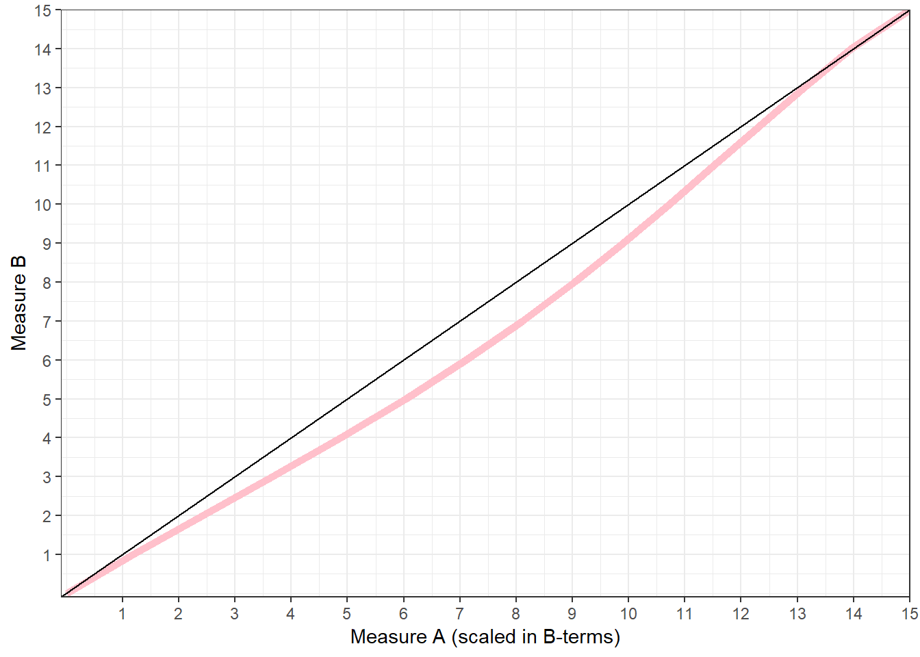
Figure 6.2: Comparison of the rescaled index A -in terms of B- with the index B.
6.5 Real-data example
For our example we will use data from the UK Family Resources Survey (FRS). This survey collects data on consensual material deprivation, drawing upon the Poverty and Social Exclusion (PSE) approach, and it is used to estimate the UK child deprivation index.
6.5.1 Step 1: Finding the anchors. MI Analysis
First we need to find the achors -invariant common items- across years. For this we will use the alligment method in Mplus to find the items that fulfill approximate MI. Warning: This analysis will take quite some time to run. On my computer, it took 5 minutes.. We already have conducted a MI analysis for the FRS data (See Chapter 5). We strongly recommend read that chapter before this one but in case you have skipped the analysis, we will run the model again.
To run the analysis we create the following MIFRS_analysis.inp file stored on the test object. The use variables command has the 17 items that are included across all years. So that we know from this subset which items could be used as anchors. Because the dimensionality of this scale is unkown, but we know that it is highly reliable, we will assume that a large part of the variance is accounted by for the higher order factor. We have 10 years, so we tell Mplus to use 10 classes to conduct the MI analysis across time points.
library(MplusAutomation)

test<-mplusObject(
  TITLE = "MI Analysis FRS data;",
  VARIABLE = "
  Names are
     gross4 FRSYear dep_ADDDEC dep_ADDEPLES dep_ADDHOL dep_ADDINS dep_ADDMEL
     dep_ADDMON dep_ADDSHOE dep_ADEPFUR dep_AF1 dep_AFDEP2 dep_HOUSHE1
     dep_CDELPLY dep_CDEPBED dep_CDEPCEL dep_CDEPEQP dep_CDEPHOL dep_CDEPLES
     dep_CDEPSUM dep_CDEPTEA dep_CDEPTRP dep_CPLAY dep_CDEPACT dep_CDEPVEG
     dep_CDPCOAT dep_ADBTBL id;
  Missing are all (-9999) ;

usevariables = dep_ADDDEC  dep_ADDHOL dep_ADDINS
      dep_ADDMON  dep_ADEPFUR dep_AF1 dep_AFDEP2 dep_HOUSHE1
     dep_CDELPLY dep_CDEPBED dep_CDEPCEL dep_CDEPEQP dep_CDEPHOL dep_CDEPLES
     dep_CDEPTEA dep_CDEPTRP dep_CPLAY;

categorical = dep_ADDDEC  dep_ADDHOL dep_ADDINS
      dep_ADDMON  dep_ADEPFUR dep_AF1 dep_AFDEP2 dep_HOUSHE1
     dep_CDELPLY dep_CDEPBED dep_CDEPCEL dep_CDEPEQP dep_CDEPHOL dep_CDEPLES
     dep_CDEPTEA dep_CDEPTRP dep_CPLAY;

classes = c(10);
knownclass = c(FRSYear = 1 2 3 4 5 6 7 8 9 10);

weight=gross4;

cluster=id;",

ANALYSIS = "type = mixture complex;
          estimator = ml;
          alignment = fixed;
          ALGORITHM=INTEGRATION;
          Process=8;",

MODEL = "
          %overall%
          f by dep_ADDDEC  dep_ADDHOL dep_ADDINS
      dep_ADDMON  dep_ADEPFUR dep_AF1 dep_AFDEP2 dep_HOUSHE1
     dep_CDELPLY dep_CDEPBED dep_CDEPCEL dep_CDEPEQP dep_CDEPHOL dep_CDEPLES
     dep_CDEPTEA dep_CDEPTRP dep_CPLAY;",
OUTPUT = "tech1 tech8 align;",

PLOT = "type = plot2;")


res <- mplusModeler(test, modelout = "MIFRS_analysis.inp",
                    writeData = "never",
                    hashfilename = FALSE,
                    dataout="FRS_mplusprep.dat", run = 1L)
The output of the MI analysis is not properly read in R. So we will simply open the MIFRS_analysis.out file and paste the summary of the MI analysis. In rows we have the Intercepts and the loadings of each item. The number corresponds to the FRS year variable in order. In brackets we have the parameters that are non-invariant for a given year. For example, the intercept of the first item is non-invariant in the first year but invariante for the rest. The second item’s threshold is invariant across all years. We see that this scale fulfills approximate measurement invariance. We appreciate that there is a subset of items that can be used as common items in that they have partial or full scalar invariance. These items are: 1,3,5,6,7,9,10,11,16 and 17.
APPROXIMATE MEASUREMENT INVARIANCE (NONINVARIANCE) FOR GROUPS

 Intercepts/Thresholds
   DEP_ADDD$1  (1) 2 3 4 5 6 7 8 9 10
   DEP_ADDH$1  1 2 3 4 5 6 7 8 9 10
   DEP_ADDI$1  1 2 3 4 5 6 7 8 9 10
   DEP_ADDM$1  (1) (2) (3) (4) 5 6 7 8 9 (10)
   DEP_ADEP$1  1 2 3 4 5 6 7 8 9 10
   DEP_AF1$1   1 2 3 4 5 6 7 8 9 10
   DEP_AFDE$1  1 2 3 4 5 6 7 8 9 10
   DEP_HOUS$1  (1) (2) 3 4 5 6 7 8 9 10
   DEP_CDEL$1  (1) (2) (3) (4) (5) 6 7 8 9 10
   DEP_CDEP$1  1 2 3 4 5 6 7 8 9 10
   DEP_CDEP$1  1 2 3 4 5 6 7 8 9 10
   DEP_CDEP$1  1 2 3 4 5 6 7 8 (9) 10
   DEP_CDEP$1  (1) 2 3 4 5 6 7 8 9 10
   DEP_CDEP$1  1 2 3 4 5 6 7 8 9 (10)
   DEP_CDEP$1  1 2 3 4 5 6 7 8 9 10
   DEP_CDEP$1  1 2 3 4 5 6 7 8 9 10
   DEP_CPLA$1  1 2 3 4 5 6 7 8 9 10

 Loadings for F
   DEP_ADDD    (1) 2 3 4 5 6 7 8 9 10
   DEP_ADDH    (1) (2) (3) (4) 5 6 7 8 9 10
   DEP_ADDI    1 2 3 4 5 6 7 8 9 10
   DEP_ADDM    1 2 3 4 5 (6) 7 8 9 (10)
   DEP_ADEP    1 2 3 4 5 6 7 8 9 10
   DEP_AF1     1 2 3 4 5 6 7 8 9 10
   DEP_AFDE    1 2 3 4 5 6 7 8 9 10
   DEP_HOUS    1 2 (3) (4) 5 6 7 8 9 10
   DEP_CDEL    1 2 3 4 5 6 7 8 9 10
   DEP_CDEP    1 2 3 4 5 6 7 8 9 10
   DEP_CDEP    1 2 3 4 5 6 7 8 9 10
   DEP_CDEP    1 2 3 4 5 6 7 8 (9) 10
   DEP_CDEP    1 2 3 4 5 6 7 8 9 10
   DEP_CDEP    (1) 2 3 4 5 6 7 8 9 10
   DEP_CDEP    1 2 3 4 5 6 7 (8) (9) 10
   DEP_CDEP    1 2 3 4 5 6 7 8 9 10
   DEP_CPLA    1 2 3 4 5 6 7 8 9 10
6.5.2 Step 2: Extract IRT parameters for each of 10 indices
Now we need the IRT parameters of the 21 items of each index. Yes, we need the full scale but remember that we have 10 anchors. We could use the MplusAutomation package to estimate the 10 models. First we need to create an iterative syntax that will run the same 2-parameter IRT for the first 7 years -they have the same items-. Then we will do the same for years 8, 9 and 10. We will save both files. The first file looks as follows:
[[init]]
iterators = i;
i = 1:7;
filename = FRS_IRT_[[i]].inp;

outputDirectory = "C:../PM Book";

[[/init]]
DATA : FILE = FRS_mplusprep[[i]].dat;

Variable:
  Names are
     gross4 FRSYear dep_ADDDEC dep_ADDEPLES dep_ADDHOL dep_ADDINS dep_ADDMEL
     dep_ADDMON dep_ADDSHOE dep_ADEPFUR dep_AF1 dep_AFDEP2 dep_HOUSHE1
     dep_CDELPLY dep_CDEPBED dep_CDEPCEL dep_CDEPEQP dep_CDEPHOL dep_CDEPLES
     dep_CDEPSUM dep_CDEPTEA dep_CDEPTRP dep_CPLAY dep_CDEPACT dep_CDEPVEG
     dep_CDPCOAT dep_ADBTBL id;
  Missing are all (-9999) ;

usevariables = dep_ADDDEC  dep_ADDHOL dep_ADDINS
      dep_ADDMON  dep_ADEPFUR dep_AF1 dep_AFDEP2 dep_HOUSHE1
     dep_CDELPLY dep_CDEPBED dep_CDEPCEL dep_CDEPEQP dep_CDEPHOL dep_CDEPLES
     dep_CDEPTEA dep_CDEPTRP dep_CPLAY dep_CDEPSUM dep_ADDEPLES dep_ADDMEL dep_ADDSHOE;

categorical = dep_ADDDEC  dep_ADDHOL dep_ADDINS
      dep_ADDMON  dep_ADEPFUR dep_AF1 dep_AFDEP2 dep_HOUSHE1
     dep_CDELPLY dep_CDEPBED dep_CDEPCEL dep_CDEPEQP dep_CDEPHOL dep_CDEPLES
     dep_CDEPTEA dep_CDEPTRP dep_CPLAY dep_CDEPSUM dep_ADDEPLES dep_ADDMEL dep_ADDSHOE;

weight=gross4;

cluster=id;


Analysis:  type = complex;
          estimator = ml;
          ALGORITHM=INTEGRATION;
          Process=8;

model:

          f by dep_ADDDEC*  dep_ADDHOL dep_ADDINS
      dep_ADDMON  dep_ADEPFUR dep_AF1 dep_AFDEP2 dep_HOUSHE1
     dep_CDELPLY dep_CDEPBED dep_CDEPCEL dep_CDEPEQP dep_CDEPHOL dep_CDEPLES
     dep_CDEPTEA dep_CDEPTRP dep_CPLAY dep_CDEPSUM dep_ADDEPLES dep_ADDMEL dep_ADDSHOE;
     f@1;


  output:
        tech1 tech8;

  plot:
          type = plot2;
The second file, for models 8, 9 and 10, looks like:
[[init]]
iterators = i;
i = 8:10;
filename = FRS_IRT_[[i]].inp;

outputDirectory = "C:../PM Book";

[[/init]]
DATA : FILE = FRS_mplusprep[[i]].dat;

Variable:
  Names are
     gross4 FRSYear dep_ADDDEC dep_ADDEPLES dep_ADDHOL dep_ADDINS dep_ADDMEL
     dep_ADDMON dep_ADDSHOE dep_ADEPFUR dep_AF1 dep_AFDEP2 dep_HOUSHE1
     dep_CDELPLY dep_CDEPBED dep_CDEPCEL dep_CDEPEQP dep_CDEPHOL dep_CDEPLES
     dep_CDEPSUM dep_CDEPTEA dep_CDEPTRP dep_CPLAY dep_CDEPACT dep_CDEPVEG
     dep_CDPCOAT dep_ADBTBL id;
  Missing are all (-9999) ;

usevariables = dep_ADDDEC  dep_ADDHOL dep_ADDINS
      dep_ADDMON  dep_ADEPFUR dep_AF1 dep_AFDEP2 dep_HOUSHE1
     dep_CDELPLY dep_CDEPBED dep_CDEPCEL dep_CDEPEQP dep_CDEPHOL dep_CDEPLES
      dep_CDEPTEA dep_CDEPTRP dep_CPLAY dep_CDEPACT dep_CDEPVEG
     dep_CDPCOAT dep_ADBTBL;

categorical = dep_ADDDEC  dep_ADDHOL dep_ADDINS
      dep_ADDMON  dep_ADEPFUR dep_AF1 dep_AFDEP2 dep_HOUSHE1
     dep_CDELPLY dep_CDEPBED dep_CDEPCEL dep_CDEPEQP dep_CDEPHOL dep_CDEPLES
     dep_CDEPTEA dep_CDEPTRP dep_CPLAY dep_CDEPACT dep_CDEPVEG
     dep_CDPCOAT dep_ADBTBL;

weight=gross4;

cluster=id;

subpopulation = FRSYear==8;

Analysis:  type = complex;
          estimator = ml;
          ALGORITHM=INTEGRATION;
          Process=8;

model:

          f by dep_ADDDEC*  dep_ADDHOL dep_ADDINS
      dep_ADDMON  dep_ADEPFUR dep_AF1 dep_AFDEP2 dep_HOUSHE1
     dep_CDELPLY dep_CDEPBED dep_CDEPCEL dep_CDEPEQP dep_CDEPHOL dep_CDEPLES
     dep_CDEPTEA dep_CDEPTRP dep_CPLAY dep_CDEPACT dep_CDEPVEG
     dep_CDPCOAT dep_ADBTBL;
     f@1;


  output:
        tech1 tech8;

  plot:
          type = plot2;
We create the *.inp files witih the createModels function using the Mplusautomation package:
createModels("FRS_IRT_models1to7.txt")
createModels("FRS_IRT_models8to10.txt")
Running the 10 2-parameter IRT models (Be patient because it will take few minutes to run all the models). We will put all the parameters on the list MI_coefs.
runModels(filefilter = "FRS_IRT_")MI_coefs<-readModels(filefilter ="frs_irt")
MI_coefs<-lapply(MI_coefs, function(x) {
x<-x$parameters$irt.parameterization
x<-x[1:42,]
x<-data.frame(a=x$est[1:21],b=x$est[22:42],c=0)
x
}
)6.5.3 Step 3: Estimating the constants for equating
We will create a list with the parameters and use the first year as reference (2013/2014). So we will constracting pairs of years were the last available year will remain fixed.
MI_coefs<-list(MI_coefs[[1]],MI_coefs[[3]],MI_coefs[[4]],MI_coefs[[5]],MI_coefs[[6]],MI_coefs[[7]],MI_coefs[[8]],MI_coefs[[9]],MI_coefs[[10]],MI_coefs[[2]])

parm_2<-cbind(MI_coefs[[1]], MI_coefs[[10]])
parm_3<-cbind(MI_coefs[[2]], MI_coefs[[10]])
parm_4<-cbind(MI_coefs[[3]], MI_coefs[[10]])
parm_5<-cbind(MI_coefs[[4]], MI_coefs[[10]])
parm_6<-cbind(MI_coefs[[5]], MI_coefs[[10]])
parm_7<-cbind(MI_coefs[[6]], MI_coefs[[10]])
parm_8<-cbind(MI_coefs[[7]], MI_coefs[[10]])
parm_9<-cbind(MI_coefs[[8]], MI_coefs[[10]])
parm_10<-cbind(MI_coefs[[9]], MI_coefs[[10]])

parm<-list(parm_2,parm_3,parm_4,parm_5,parm_6,parm_7,parm_8,parm_9,parm_10)
comitems<- c(1,3,5,6,7,9,10,11,16,17)
We now use the function irt.link() from the package SNSequate to find the equating parameters “a” and “b” using 2013/3014 as reference year, i.e. all the deprivation scores will be in terms of 2013/2014.
eqconst<-lapply(1:9, function(i) irt.link(parm[[i]], comitems, model = "2PL", icc = "logistic", D = 1.7))Once we have found the parameters we can extract them. For this example we will use the Haebara estimates for this example. Yet, you could check by yourself that there are very minimal using other methods.
H<-do.call("rbind", lapply(eqconst, "[[", 4))
H<-split(H, seq(nrow(H)))
6.5.4 Step 4: Applying the constants and obtaning equated scores
We need then to apply the constants to each IRT-coefs dataset
FRSIRT <- MI_coefs[2:10]

parm.x<-lapply(1:9, function(i) {
  FRSIRT[[i]]$a<-FRSIRT[[i]]$a/H[[i]][1]
  FRSIRT[[i]]$b<-H[[i]][1]*(FRSIRT[[i]]$b)+H[[i]][2]
  FRSIRT[[i]]
} )theta_points=c(-5,-4,-3,-2,-1,0,1,2,3,4,5)
param_x<-lapply(parm.x[1:9], function(x) list(a=x$a,b=x$b,c=x$c))
param_y<-lapply(1:9, function(x) list(a=MI_coefs[[1]]$a,b=MI_coefs[[1]]$b,c=MI_coefs[[1]]$c))
true_eqscale<-lapply(1:9, function(i) irt.eq(21, param_x[[i]], param_y[[i]], method="TS", A=1, B=0, common=comitems))
obs_eqscale<-lapply(1:9, function(i) irt.eq(21, param_x[[i]], param_y[[i]], theta_points, method="OS", common=comitems,
A=1, B=0))Observed score equating. We observe that despite the changes to the child deprivation score, the scale is very stable across years. There are minor differences across years when we round the numbers. We appreciate, however, that the years 2007-2011 show substative differences relative to 2013/2014. Particularly, among the severely deprived population. For the same latent severity of poverty, a deprivation scroe equal to 8 in 2009/2010 is equal to a score of 9 in 2013/2014.
obs_mean<-lapply(obs_eqscale, function(x) data.frame(score.xiny=x$e_Y_x))
obs_mean<-as.data.frame(obs_mean)
names(obs_mean)<-c("2004/2005","2005/2006","2006/2007","2007/2008","2008/2009","2009/2010","2010/2011","2011/2012",
                   "2012/2013")
obs_mean$Reference<-0:21
round(obs_mean,0)
## 2004/2005 2005/2006 2006/2007 2007/2008 2008/2009 2009/2010 2010/2011
## 1 -1 -1 -1 -1 -1 -1 -1
## 2 1 1 1 2 2 1 1
## 3 2 2 3 3 3 2 2
## 4 3 4 4 4 4 3 3
## 5 4 5 4 4 4 4 4
## 6 5 6 5 5 4 4 5
## 7 6 6 6 6 5 5 6
## 8 7 7 7 7 6 6 7
## 9 8 8 8 8 7 7 9
## 10 9 9 9 9 8 8 10
## 11 10 10 10 10 9 9 11
## 12 11 11 11 10 10 10 12
## 13 12 12 12 11 11 11 14
## 14 13 13 13 12 12 12 15
## 15 14 14 14 13 13 13 16
## 16 14 15 15 14 14 15 16
## 17 15 16 16 15 15 16 17
## 18 17 17 17 16 16 17 18
## 19 17 18 18 17 17 18 19
## 20 18 19 19 18 18 19 19
## 21 19 20 19 19 19 19 20
## 22 21 21 21 20 20 21 21
## 2011/2012 2012/2013 Reference
## 1 -1 -1 0
## 2 1 1 1
## 3 2 2 2
## 4 3 3 3
## 5 4 4 4
## 6 5 5 5
## 7 6 6 6
## 8 7 7 7
## 9 8 8 8
## 10 9 9 9
## 11 11 10 10
## 12 12 12 11
## 13 15 13 12
## 14 16 14 13
## 15 16 15 14
## 16 17 16 15
## 17 18 17 16
## 18 19 18 17
## 19 19 19 18
## 20 20 20 19
## 21 20 20 20
## 22 21 21 21Plotting the results. See plot @Ref(fig:frsobseq)
library(reshape2)
mm<-melt(obs_mean, id="Reference")

ggplot(mm,aes(x=Reference,y=value, group=variable, colour=variable)) + geom_line(aes(linetype=variable), size=2) +
  xlab("2013") + ylab("Rescaled") + theme_bw() +    scale_y_continuous( limits = c(-1.5,8),  breaks = seq(-2, 8, 1) ) +
  geom_abline(slope=1, intercept=0) + theme(legend.position="bottom") +
  scale_x_continuous( limits = c(-1.5,8), breaks = seq(-2, 8, 1))
## Warning: Removed 123 rows containing missing values (geom_path).
Figure 6.3: Comparison of the rescaled indices. Reference year: 2013/2014
6.5.5 Finding equated poverty lines
Now that we have put deprivation scores in terms of the reference year, we can estimate poverty using adjusted poverty lines. This will help us to assess how poverty changes when we used a fixed poverty line relative to when we use a equated one. The adjusted poverty line transforms the value of reference, lets say 3, into an adjusted value, i.e. what is 3 in a given year in terms of 2013/2014. To asses this, first we will paste the adjusted deprivation scores by year. So we will creata the mm data frame.
library(reshape2)

mm$FRSYear[mm$variable=="2004/2005"]<-1
mm$FRSYear[mm$variable=="2005/2006"]<-2
mm$FRSYear[mm$variable=="2006/2007"]<-3
mm$FRSYear[mm$variable=="2007/2008"]<-4
mm$FRSYear[mm$variable=="2008/2009"]<-5
mm$FRSYear[mm$variable=="2009/2010"]<-6
mm$FRSYear[mm$variable=="2010/2011"]<-7
mm$FRSYear[mm$variable=="2011/2012"]<-8
mm$FRSYear[mm$variable=="2012/2013"]<-9
mm$FRSYear[mm$variable=="2013/2014"]<-10
mm$ds_uw<-mm$Reference
Now we can merge the mm data with the FRS_mplusprep.dta file. We will crate a deprivation score considering the 21 indicators for each year (remember that in 2012 the indicators changed). We will call this deprivation score ds_uw(unweighted). Then we marge the mm data with the FRS_mplusprep.dta data and assign the ds_uw to the 2013/3014 data (as it is not present in the mm file).
library(haven)

D<-read_dta("FRS_mplusprep.dta")

if(D$FRSYear<=7) {
  D$ds_uw<-rowSums(D[,c(3:23)],na.rm=TRUE)
} else {
  rowSums(D[,c(3,5,6,8,10,11:19,21:27)],na.rm=TRUE)
}
## Warning in if (D$FRSYear <= 7) {: the condition has length > 1 and only the
## first element will be usedD<-merge(D,mm,by=c("FRSYear","ds_uw"),all.x=T)
D$value[D$FRSYear==10]<-D$ds_uw## Warning in D$value[D$FRSYear == 10] <- D$ds_uw: number of items to replace
## is not a multiple of replacement lengthThe next step is to create a column to identify who is poor and who is not based on the unadjusted and adjusted poverty line. We will use \(3\) as the value of the poverty line in this example -See Chapter XX for a discussion of the poverty line-. To get the adjusted poverty lines we need to get the rows for each year that are equal to (unadjusted 3).
D2<-subset(D,D$ds_uw==3)
lines<-ddply(D2,.(FRSYear), summarise, mean=mean(value))
lines
## FRSYear mean
## 1 1 3.4970670
## 2 2 3.5258663
## 3 3 3.5630543
## 4 4 3.5485614
## 5 5 3.5729468
## 6 6 3.4339168
## 7 7 3.4580138
## 8 8 3.1552975
## 9 9 3.3381506
## 10 10 0.9195776Now all we have to do is to merge the files and identify poverty using the thresholds equal to 3 for both the adjusted and the unadjusted poverty line.
D<-merge(D,lines,by="FRSYear")
D$mean<-round(D$mean)
D$mean[D$FRSYear==10]<-3

D$poor_uw<-ifelse(D$ds_uw>=3,1,0)
D$poor_w<-ifelse(D$ds_uw>=D$mean,1,0)
We will do a simple calculation of the prevalence rate for each year using both poverty lines. We will simply consider the survey weights in this occasion. The function svyby will give us both the point estimate and the standard errors. We will produce the bands of the confidence intervals (95%) for the plots below.
library(survey)

des<-svydesign(id=~1, weights=~gross4, data=D)

pov_uadj<-svyby(~poor_uw, ~FRSYear, des, svymean)
pov_adj<-svyby(~poor_w, ~FRSYear, des, svymean)
pov_adj<-merge(pov_adj,pov_uadj,by="FRSYear")
pov_adj<-pov_adj[,c(2:ncol(pov_adj))]*100
pov_adj$ci_wu<-pov_adj$poor_w+1.96*(pov_adj$se.x)
pov_adj$ci_wl<-pov_adj$poor_w-1.96*(pov_adj$se.x)
pov_adj$ci_uwu<-pov_adj$poor_uw+1.96*(pov_adj$se.y)
pov_adj$ci_uwl<-pov_adj$poor_uw-1.96*(pov_adj$se.y)


pov_adj$year<-c("2004/2005","2005/2006","2006/2007","2007/2008","2008/2009","2009/2010","2010/2011","2011/2012",
                   "2012/2013","2013/2014")
After we produce the relevant calculations we can plot the evolution of child poverty with confidence intervals (95%) using both lines using ggplot2. The adjusted poverty line indicates that prior the economic crisis there was a drop in child poverty and that it has decreased after 2011/2012. The unadjusted measure shows very low variability and see that the change to the set of indicator does not seem to impact the prevalence rate (yet, it does so in terms of severity).
p1<-ggplot(pov_adj,aes(y=poor_w, x=year, group=1))  + geom_line(aes(color="green")) + geom_ribbon(aes(ymin=ci_wu, ymax=ci_wl), fill="green", alpha=.4) + ylab("% Child poverty") +
    scale_y_continuous( limits = c(20,40),  breaks = seq(20, 40, 5) ) + theme_bw()

p2<-p1 + geom_line(aes(y=poor_uw, x=year, group=1, color="#F5A9A9")) + geom_ribbon(aes(ymin=ci_uwu, ymax=ci_uwl), fill="#F5A9A9", alpha=.4) + theme_bw() + scale_color_discrete(name = "Poverty line", labels = c("Unadjusted", "Adjusted"))
p2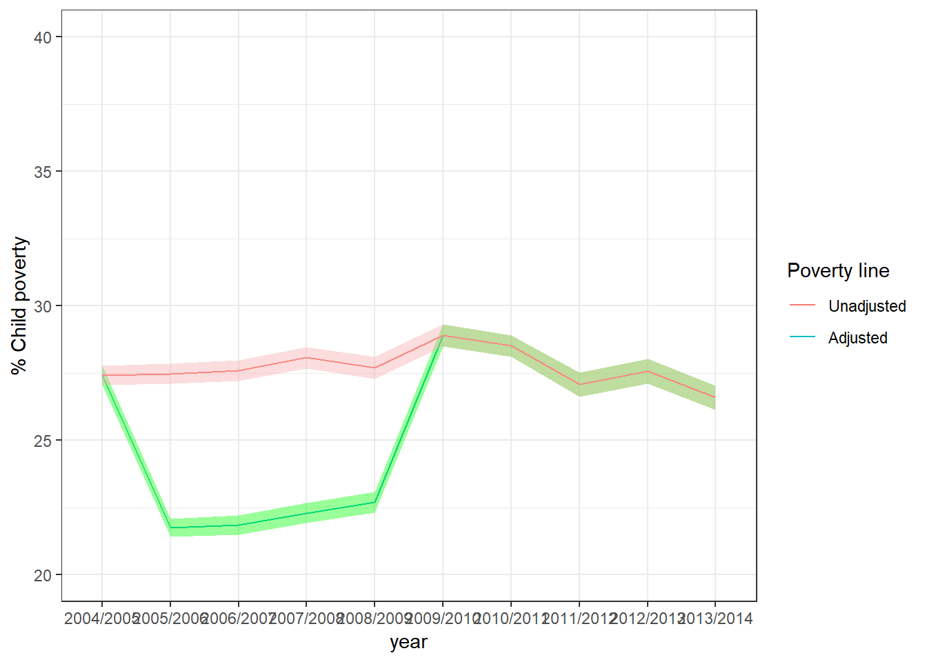
Figure 6.4: Evolution of the child poverty in the UK. 2004-2014. Adjusted ppoverty lines. Reference year: 2013/2014